Why the Cheapest Cable and Magnet Cost the Most
A plant will approve a serious analyser and then defeat it with an unspecified cable and an unknown magnet. This is the commercial case for buying the whole measurement chain to a specification — the three failure modes that cost real money, the questions that separate a measurement-grade accessory from a generic one, and an interactive model you can drive with your own numbers.
You do not buy an analyser. You buy a chain.
- Every link in the measurement chain is in series, so the reading is defined by the cheapest one.
- By the time a number reaches the analyst, nothing in it says which link changed.
- The usual purchasing pattern evaluates the DAQ technically and buys the cable and mount through stores — which throws away the specification you paid for.
A vibration reading is not produced by an instrument. It is produced by a chain: the sensor, the mount that couples it to the machine, the cable that carries the charge or the voltage, the conditioning that powers the sensor, the DAQ that digitises it, and the analysis that turns the digits into a verdict. Every one of those links is in series. The number that reaches the analyst has already passed through all of them, and by then there is nothing in the number that says which link changed.
This is why the usual purchasing pattern is so damaging. The DAQ and the software go through a technical evaluation, because they are the visible, expensive line items. The cable and the mount go through the stores, because they are consumables. A plant will sign for a four-channel 24-bit analyser and then connect it with a cable bought on price alone and a magnet whose only stated property is that it is a magnet. The chain is now defined by its cheapest link, and the specification of the expensive one has been thrown away.
The rest of this article is not about which brand to buy. It is about three specific ways a weak link costs money — false alarms, missed faults and lost trend history — the questions that let you tell a specified accessory from an unspecified one, and an honest, editable model you can run on your own machine count and your own downtime rate. The physics behind each link is covered in three companion articles, linked below.
Failure mode one: false alarms
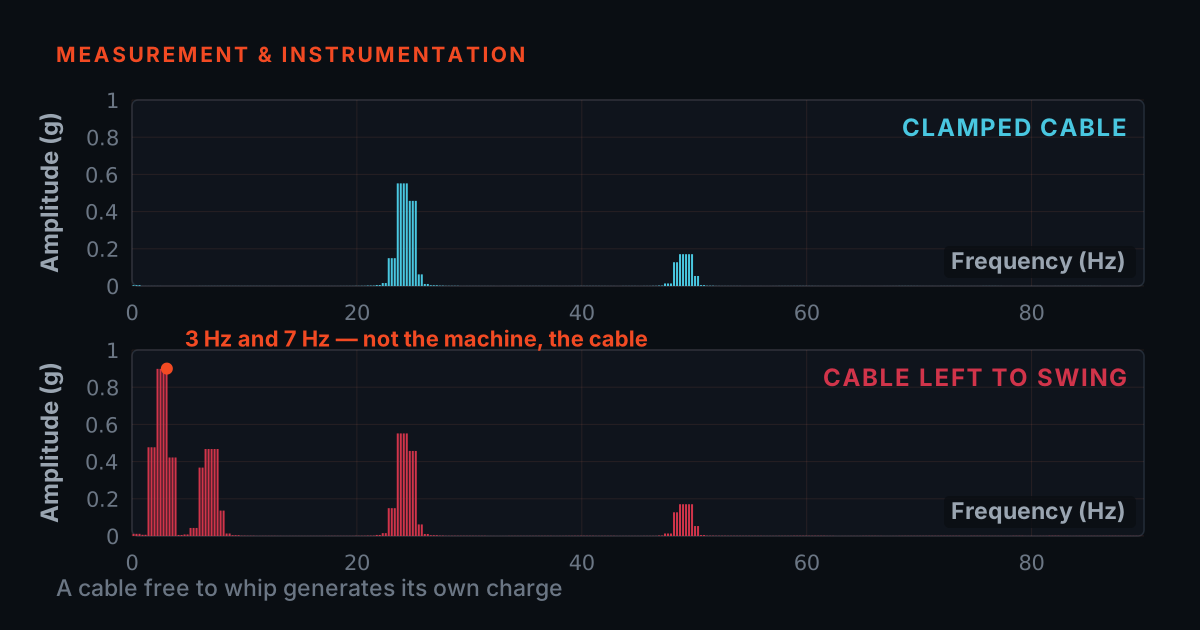
A cheap cable does not fail silently. It generates signal. Coaxial cable that flexes under machine vibration produces triboelectric noise — charge released as the dielectric separates from the shield, appearing at the input as a voltage the sensor never produced. A poorly clamped connector adds intermittent contact noise. A magnet that rocks on a curved or painted surface adds impact chatter of its own. A noisy DAQ input adds a floor that never goes away. None of that is the machine, and all of it looks exactly like the machine to a threshold.
The immediate cost of a false alarm is a stopped machine and a strip-down that finds nothing wrong. That is a bad afternoon. The second-order cost is worse and it is permanent: the crew learns that the system cries wolf. After the third healthy machine is opened, the alarms stop being acted on, and the day a real alert fires it is read as another cable problem. A condition-monitoring programme that is no longer believed is not a programme with a fault. It is a programme with no output, still being paid for.
The engineering test for this failure mode is simple. Take a reading with the machine stopped. Take another with the machine running but the sensor held off the machine. Flex the cable by hand during a measurement and watch the spectrum. If any of those produce signal you would have alarmed on, the alarm you saw last week may never have come from the bearing.
Failure mode two: the fault you bought the programme to catch
- An early bearing defect is a small, high-frequency signal sitting next to a large, low-frequency one, and it has to survive two separate hurdles to reach the analyst.
- The mount decides whether the bearing tones are still inside the usable band; the cable and DAQ noise floor decide whether a small peak still stands above it.
- Fail either one and the analyser reports the only thing left in the band, which is the running-speed peak.
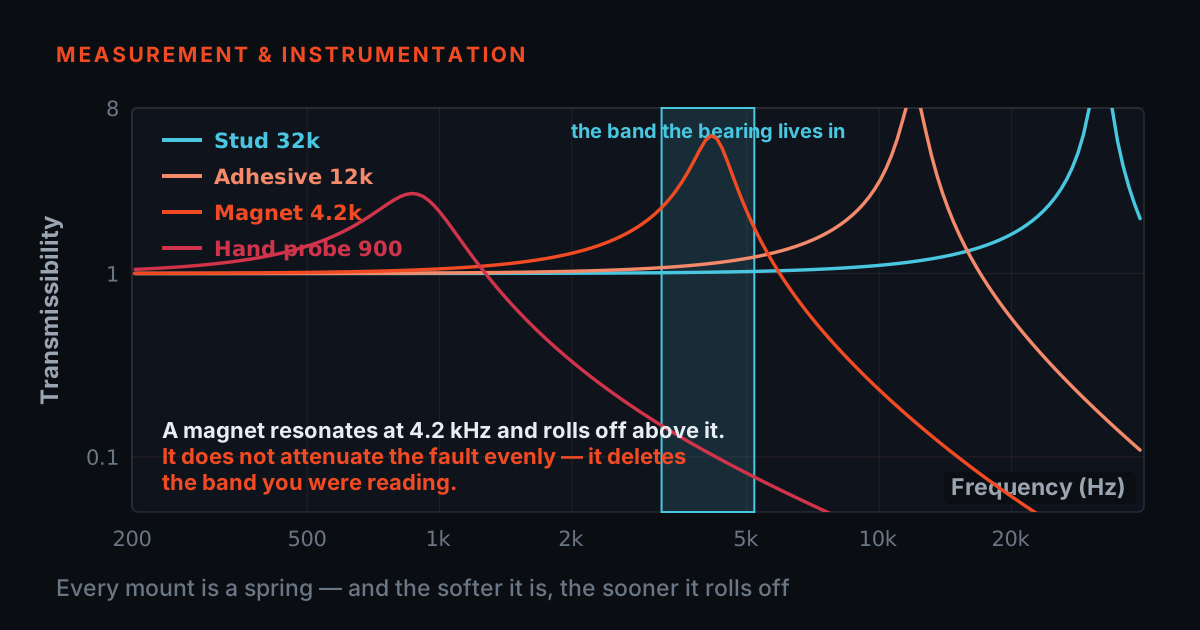
The second failure mode is quieter, and that is what makes it expensive. An early bearing defect is a small, high-frequency signal sitting next to a large, low-frequency one. It has to survive two things to reach the analyst: the mounted resonance of the sensor-and-mount assembly has to be high enough that the bearing tones are still inside the usable band, and the noise floor of the cable and the DAQ has to be low enough that a small peak still stands above it.
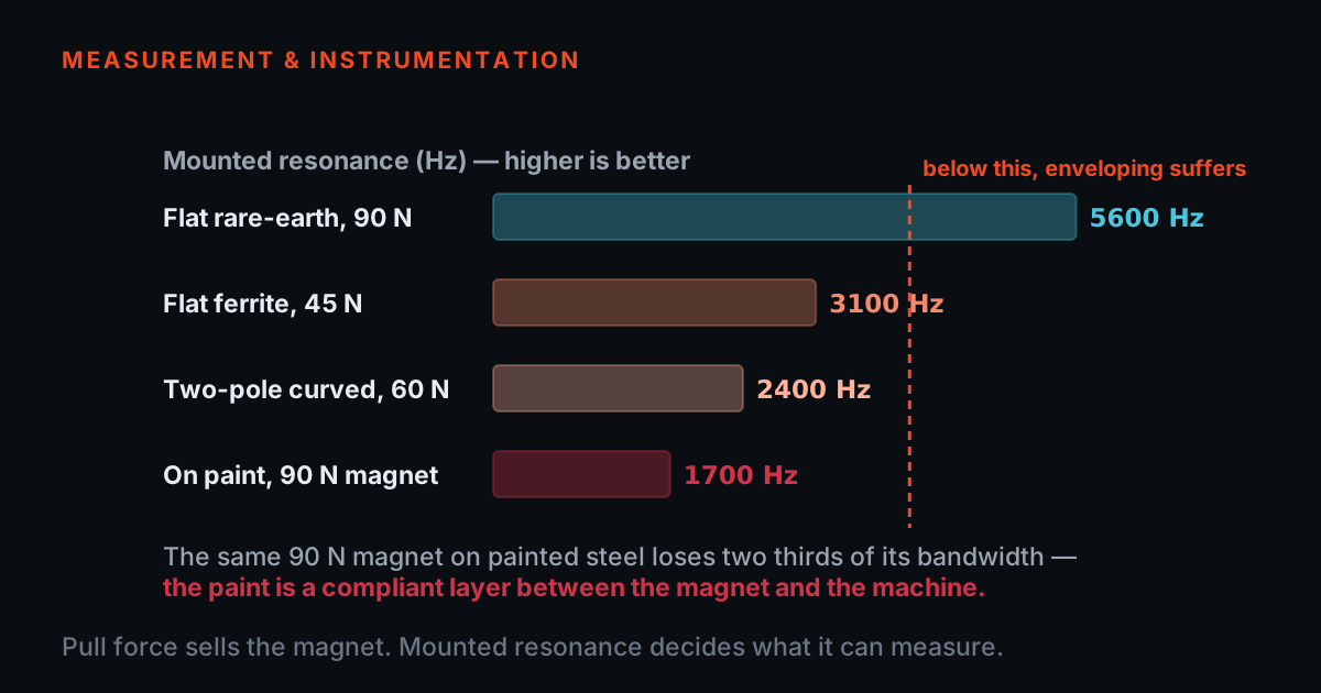
A magnet lowers the mounted resonance because it inserts a compliance between the sensor and the machine. A large flat magnet on a rough painted surface lowers it further. Once the usable band ends below the bearing tones, the analyser is not reading a healthy bearing — it is reading a bearing it cannot see, and reporting the only thing left in the band, which is the running-speed peak. The trend looks flat and reassuring right up to the failure. The mount article covers where that resonance lands and why; this article is only concerned with what it costs.
The noise floor does the same job by a different route. A defect that produces a peak of one hundredth of a g is plainly visible above a floor of one thousandth and completely invisible against a floor of one twentieth. Nothing in the software will tell you the peak was there and got buried. The spectrum simply comes back clean, and a clean spectrum from a bad chain is indistinguishable from a clean spectrum from a healthy machine. Drag the slider below and watch the same growing defect appear in one chain and not in the other.
A synthesised illustration, not measured data. The defect signal is identical in both panels. Only the noise floor and the mount roll-off differ.
Failure mode three: the trend stops being comparable
The output of a condition-monitoring programme is not a reading. It is a trend. A single number in isolation tells you very little; the same point measured the same way every month tells you almost everything, because the machine is being compared against itself. That comparison only holds while nothing except the machine has changed.
Three things break it quietly. Inconsistent mounting: a magnet placed a few centimetres away, or on paint this month and bare metal last month, changes both the level and the usable bandwidth. Drifting sensitivity: an uncalibrated sensor whose output has moved five per cent since last year puts a five per cent slope into a trend that nothing in the plant caused. And a changed cable: a replacement with different capacitance and a different noise floor shifts the baseline on the day it is fitted.
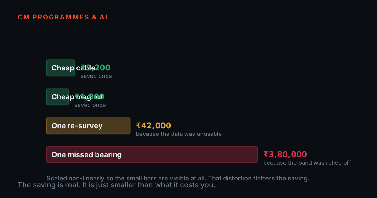
The cost is specific and it is not recoverable. When the trend steps, you cannot tell whether the machine changed or the hardware did, so the alert levels derived from the old data are void and the history before the change has to be discarded. You are back to month one on that machine, and the twelve months of data you paid technicians to collect bought nothing. The saving on the replacement cable was three hundred rupees. The cost was a year of history on every point it touched.
Try it: the cost of a weak link
This calculator does not know your plant, and it is not a study. It is arithmetic on assumptions, and every assumption it uses is printed below the controls where you can see it and change it. Set your machine count, your points, your downtime rate and the length of a typical unplanned stop, then choose a quality tier for each of the three links. It compares a fully specified chain against the chain you chose, and puts the hardware saving next to the consequences.
The tier logic is deliberately crude, because a defensible crude model is more useful than an impressive one you cannot check. Each link earns weak-link points — three for a generic, unspecified item, one for a mid-grade commercial item, none for a measurement-grade item with published figures. Those points raise the false-alarm rate and lower the probability that an early fault is detected in time. Both effects are linear, both rates are editable, and both defaults are engineering judgement rather than measurement.
Read the output as a shape, not as a number. If you halve every assumption the conclusion generally survives, and that is the only claim this model makes: the hardware saving happens once, and the consequence of a weak chain repeats every year at several times its size. Change the assumptions until you believe them, then look at the two bars again.
| Indicative annual outcome | Specified chain | Your chain |
|---|
Assumptions — every one of them is editable, and none of them is measured data
These are the rates the arithmetic above uses. They are engineering judgement chosen to be plausible, not observations from any plant, any customer or any test programme. Change them to whatever you can defend from your own records; the table and the bars update as you type.
Hardware prices, in rupees per item. Round illustrative figures for the arithmetic — not quotations, and not the price of any particular product. Replace them with your own quotes.
Two further modelling choices, stated so they are not hidden: one kit is counted as one DAQ, one cable and one mount; and a fault that is detected is assumed to be repaired in a planned window, contributing no unplanned hours, while a fault that is missed costs one unplanned stop of the length you set above.
Ask for the number
- A supplier who has tested a component quotes it with units and test conditions. One who has not answers with adjectives.
- The published number is what you are buying — it is what lets you design around a limitation and say so on the report.
- Ask for a traceable calibration certificate for the sensor and a batch or unit test record for the accessory.
There is one test that separates a measurement-grade accessory from a generic one, and it does not require a laboratory. Ask for the number. A supplier who has tested a component can quote it with units and test conditions. A supplier who has not will answer with adjectives — high quality, industrial grade, suitable for vibration. Adjectives are not a specification, and a component with no specification is an unknown that you are about to install permanently in your measurement chain.
This is not about brand loyalty and it is not about price. A cheap component with a published, honest specification is a known quantity, and a known quantity can be designed around: if the mounted resonance is 3 kHz you simply do not trust the spectrum above about 1 kHz, and you say so on the report. An expensive component with no published specification is still an unknown. The number is what you are buying.
One more question that is worth more than all of them: is there a traceable calibration certificate for the sensor this accessory serves, and a batch or unit test record for the accessory itself? Traceability is what lets you say that the reading you took last March and the reading you took this March mean the same thing. Without it, a trend is a collection of numbers that happen to be on the same chart.
| Item | Ask for this number | What it protects |
|---|---|---|
| Cable | Noise figure under flex, and capacitance per metre | The noise floor your small early peaks have to stand above |
| Cable | Temperature rating of jacket and connector | Whether the reading survives a hot bearing housing in May |
| Mount | Pull-off force, quoted perpendicular and in shear | Whether the magnet stays put on a vertical or curved surface |
| Mount | Mounted resonance with a stated sensor mass and surface | The usable upper frequency — where bearing tones live |
| DAQ | Input noise floor and dynamic range, at a stated range setting | Whether a small peak survives beside a large 1× peak |
| Whole chain | Batch test record, and a traceable calibration certificate for the sensor | That the item you received is the item that was tested |
When the cheap accessory is the right answer
It would be dishonest to stop there, because the cheap option is sometimes correct, and pretending otherwise makes the rest of this article a sales pitch. The argument above is about trended condition monitoring. Where you are not trending, most of it does not apply.
A one-off rough check is a good example. An operator reports that a pump sounds different, someone walks over with a meter, and the question is whether the level is two millimetres per second or twenty. That decision survives a great deal of noise and a mediocre mount, because the answer is an order of magnitude, not a trend. The same is true of a quick comparison between two identical machines running side by side on the same day: whatever the chain does wrong, it does to both.
A training rig is another. On a fault simulator you already know what fault is present, the amplitudes are large by design, and the purpose is to teach a technician to recognise a pattern. A modest cable and a plain magnet teach that pattern perfectly well, and spending the training budget on measurement-grade accessories instead of on more hours at the rig is a poor trade.
The rule that separates the two cases is simple. If the reading will be compared — against last month, against a threshold, against a sister machine measured at another time — buy the specification. If the reading will be used once, looked at, and thrown away, buy what is convenient. The mistake is not owning a cheap accessory. The mistake is letting a cheap accessory into a trend without noticing.
- Buy the specification wherever the reading will be compared — against last month, a threshold, or a sister machine measured at another time.
- Buy what is convenient for a one-off rough check where the answer is an order of magnitude.
- Use a modest cable and a plain magnet on a training rig, and spend the difference on hours at the rig.
- Compare two identical machines side by side on the same day with whatever chain you have — the errors apply to both.
- Do not let an unspecified accessory into a trended point without recording that you did.
- Do not buy measurement-grade accessories for a fault simulator where the amplitudes are large by design.
- Do not treat a walk-over rough check as if it set a baseline.
- Do not assume the rule is about price — it is about whether the reading will be compared.
Where TIERA fits, factually
TIERA supplies the whole chain rather than one part of it: IEPE accelerometers, low-noise coaxial and armored cables, magnetic mounts and SS304 triaxial blocks, adhesive pads, junction boxes, PhonoVibe DAQs and TVIB analysis software. Individual datasheets for the cables and mounts are published in the public TIERA datasheets repository, which exists precisely so that a buyer can read the specification before raising the purchase order rather than after.
Two links in that chain carry calibration documents. Every PhonoVibe DAQ ships with a factory calibration certificate carrying one year of validity. The T-Calibro back-to-back calibrator lets a plant verify accelerometer sensitivity on its own bench, and its reference sensor ships with a factory calibration certificate establishing its sensitivity against a national-standard traceable chain. That is what makes a trend comparable across years rather than merely across months.
The claim is a modest one and it is worth stating precisely. Buying the chain from one supplier does not make the measurement good on its own — mounting discipline and a competent analyst matter at least as much. What it does is remove the unknowns: the cable has a published construction, the mount has a published pull-off force, the DAQ has a published resolution and a calibration certificate, and the sensor has a sensitivity you can verify. When the trend then moves, you can be reasonably confident it moved because the machine did.
TIERA instruments that do this work.

Sensors & Accessories
The links this post is about — cable, mount and sensor — each supplied with its own datasheet rather than as an unspecified consumable.
- Cables
- Low-noise coaxial CA-101 (10-32/M5 to BNC) against triboelectric noise; CA-102 2-core twisted shielded (MIL to BNC); armored SS outer CA-103 — 5 m standard
- Mounts
- TMA-101-1 magnetic mount (SS 304); TMB-101-1-A SS304 triaxial mounting block; TAP-101-1A adhesive pad set
- Accelerometers
- TACPB-10T3 uniaxial MEMS IEPE, plus industrial, compact and low-frequency variants
- Routing
- Vibration junction boxes for clean cable routing on multi-point tests
- Documentation
- Individual datasheets for every cable and mount in the public datasheets repository

PhonoVibe Series — Sound & Vibration DAQ
The DAQ link, bought with its numbers stated: resolution, sensor power, bandwidth and a calibration certificate in the box.
- ADC resolution
- 24-bit across the entire series
- PhonoVibe D
- 2 channel · 48 kHz · 2 Hz – 20 kHz · ±10 V input
- PhonoVibe Q
- 4 channel · 128 kHz · 0.5 Hz – 60 kHz · ±5 V input
- Sensor power
- IEPE / ICP / CCLD — 24 V, 4 mA constant current; TEDS supported
- Calibration
- Factory calibration certificate, 1-year validity

T-Calibro Vibration Calibration System
The answer to drifting sensitivity — verify the sensor on your own bench and keep an audit-ready record, so this year's trend is comparable with last year's.
- Method
- Back-to-back comparison calibration
- Calibration frequency
- 159.2 Hz (≈1000 rad/s), per ISO 16063 back-to-back convention
- Compatibility
- All IEPE / ICP accelerometers
- Records
- Automated calibration record — date, operator, conditions, before/after sensitivity — with one-click certificate export
- Certificate
- Factory calibration certificate included with the unit
From the TIERA store
The kit for this job
What we would actually put in front of someone doing the measurement this post describes — not the whole catalogue.
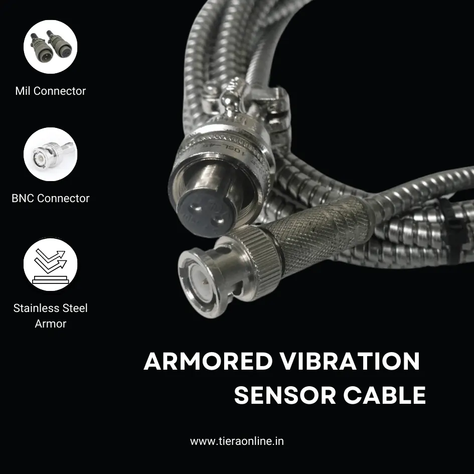 Armored Vibration sensor cableCA-103-5-A : Tinned Copper Braid 2 Core Twisted Shielded Cable with Stainless Steel Outer Armor – One side 2 pin Circular MIL Connector other side Bare wires / BNC Connector₹2,300View →
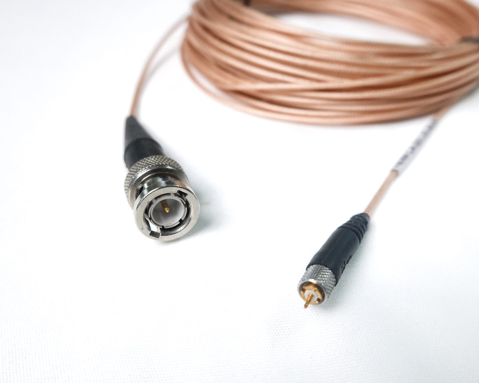 Low-Noise Coaxial Sensor CableCA-101-5-M-B: Low-Noise Tin plated copper braid Coaxial cable – one end 10-32 / M5 Microdot Connector other end BNC Connector₹2,200View →
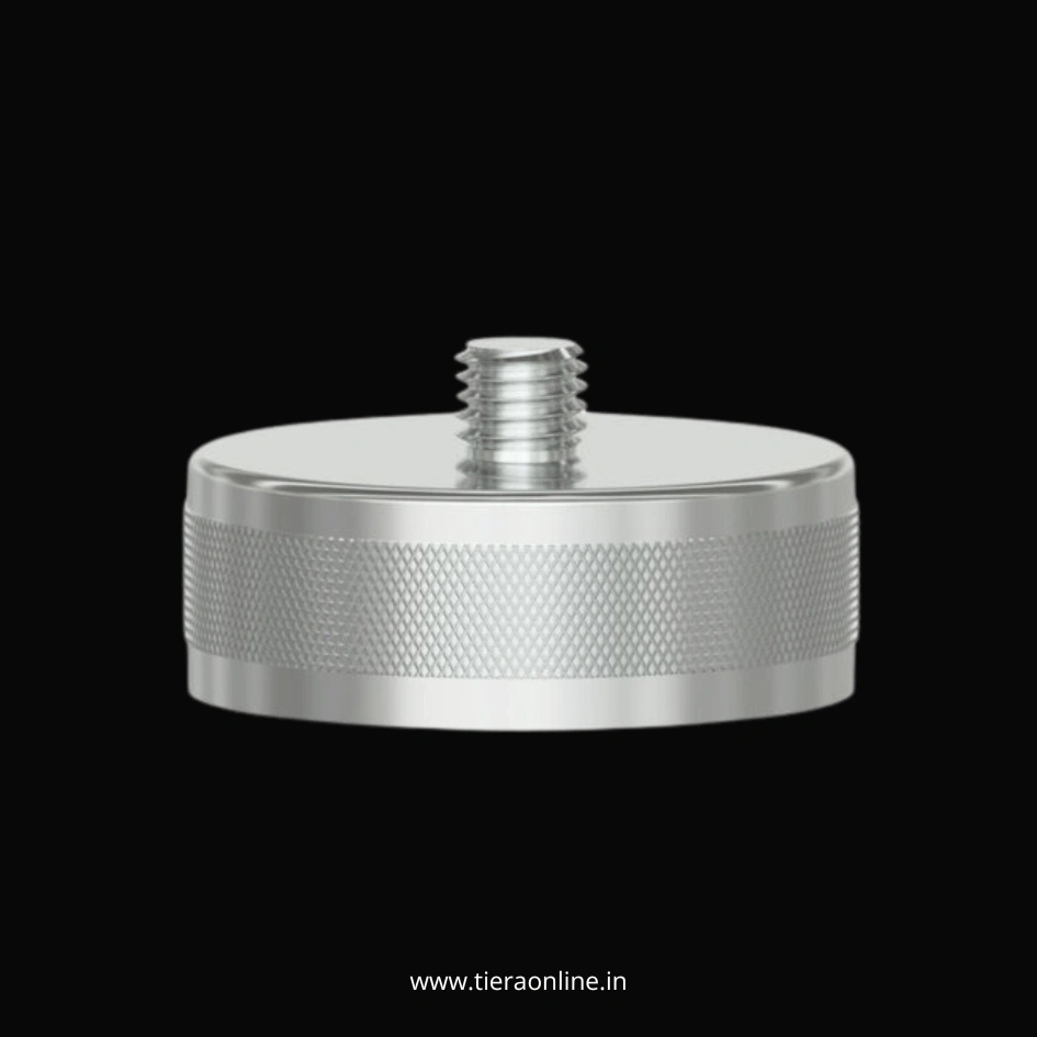 Magnetic Mounting Pad for Vibration sensorTMA-101-1A : SS 304 Magnetic Mount for Accelerometers and Vibration Sensors.₹800View →
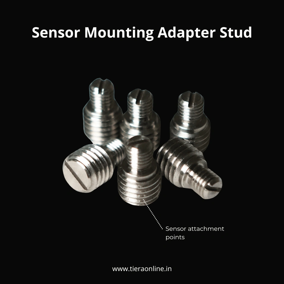 Sensor Mounting Adapter StudTM101-1A : TIERA SS304 Adapter Stud for sensor mounting₹260View →
Use cases
Where this shows up in the field
Buy the chain with its numbers attached, not the box with the biggest label.
TIERA supplies every link between the machine and the verdict: IEPE accelerometers, low-noise coaxial and armored cables, magnetic mounts, SS304 triaxial blocks and adhesive pads, junction boxes, PhonoVibe 24-bit DAQs and TVIB analysis software. The cables and mounts have individual datasheets in the public TIERA datasheets repository, so the specification is available before the purchase order rather than after the first strange reading.
If you are specifying a route kit and want the chain checked as a chain, send us the machine list and the points you intend to trend. Our engineers will tell you which links your programme genuinely needs at measurement grade and which ones it does not — including the cases where the cheaper item is the correct answer.
- Cables with a stated construction — low-noise coaxial CA-101 against triboelectric noise, CA-102 twisted shielded, and armored SS-outer CA-103 for runs near moving machinery, 5 m standard.
- Mounts with published datasheets — TMA-101-1 SS 304 magnetic mount for walk-around routes, TMB-101-1-A triaxial block and TAP-101-1A adhesive pads for permanent marked points.
- PhonoVibe DAQs — 24-bit, simultaneous sampling, IEPE/ICP/CCLD sensor power at 24 V and 4 mA, each shipping with a factory calibration certificate valid for one year.
- T-Calibro back-to-back calibrator — verify accelerometer sensitivity on your own bench and export the certificate, so a five-year trend stays comparable across its whole length.
Where this sits on the TIERA learning ladder.
The theory behind this article is covered free, in full, by the TIERA 101 primers: Measurement Setup 101, Accelerometer & DAQ Selection 101. They are self-paced, interactive, and end in an exam and a certificate.
The free primers teach a technician why mounting and cabling change the reading; TCAT (Category I to IV, with proctored examinations) builds the analyst who can defend a measurement decision to a plant manager.
TIERA 101 is a free introductory primer, not an accredited ISO certification, and its hours do not count towards the formal training ISO 18436 requires.