The Magnet That Deleted a Bearing Fault
How you attach the sensor decides which frequencies you are allowed to see. A mini explainer plus a live simulator: pick stud, adhesive, magnet or probe, drag a fault frequency, and watch an early bearing tone vanish.
A fault can be real and still invisible
- The mechanical joint between machine and sensor is a filter, and it acts before the electronics, the DAQ and every software setting you can inspect.
- A frequency the joint does not pass cannot be recovered by gain, averaging or any FFT option.
- Two clean spectra from the same bearing on the same day can mean completely different things.
An accelerometer does not measure the machine. It measures whatever motion makes it through the mechanical joint between the machine and the sensor base — the stud, the glue, the magnet, or the pressure of a hand on a probe. That joint is a filter, and it is applied before the electronics, before the DAQ, before any software setting you can inspect. If the joint does not pass a frequency, no gain knob or FFT option will bring it back.
This is why two technicians can survey the same bearing on the same day and file opposite reports. One screwed the sensor into a spot face; the other slapped a magnet on painted steel. Both saw a clean spectrum. Only one of those spectra was allowed to contain the fault.
Every mount is a spring, and every spring has a resonance
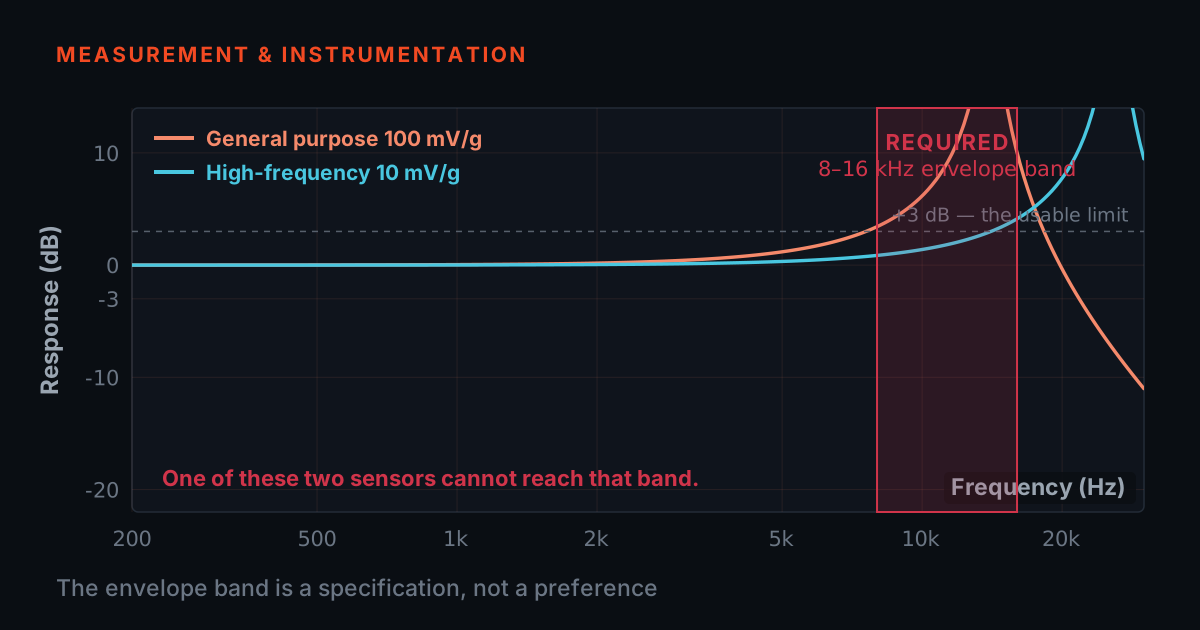
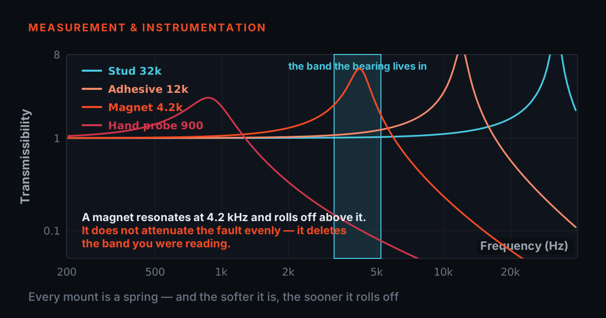
Mechanically, sensor-on-mount is a mass on a spring: the accelerometer's mass sitting on the stiffness of the joint. Like every mass-spring system it has a natural frequency — the mounted resonance. Below it, the sensor follows the surface faithfully and the response is flat: this is the band you can trust. Approaching it, the joint amplifies motion and readings lift, sometimes by 10–20 dB — numbers there are exciting and wrong. Above it, the sensor stops following the surface at all and the response collapses at roughly 40 dB per decade — frequencies up there simply do not arrive.
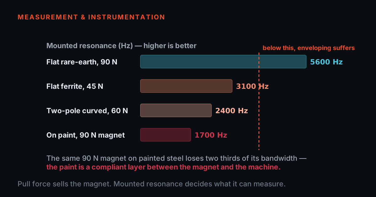
A stiff joint pushes the resonance high and the collapse far away; a compliant joint drags both down into the frequencies you care about. A stud is metal-to-metal and stiff. Glue is softer. A magnet is a stiff element gripping through whatever sits under it — paint, scale, curvature — so its effective stiffness is set by the worst layer in the stack. A hand on a probe is the softest spring in the building. The common rule of thumb — and it is a rule of thumb, not a law — is to trust the region up to roughly one-third of the mounted resonance, where the resonance has lifted the reading by only about 1 dB (some 10–12 percent); houses that need tighter amplitude accuracy use one-fifth, which keeps the lift under about 5 percent. The datasheet quotes the stud-mounted resonance; for magnets and pads the effective resonance depends on the surface under them, so on a critical point it should be measured — a simple bump test shows the peak — not assumed.
Try it: the mounting bandwidth simulator
The simulator below draws the mounting frequency response for four methods and overlays a fault tone you position. The grey bar is the tone as it exists on the machine; the orange bar is what your mount lets you record. Start on stud with the early bearing tone at 9.5 kHz — inside the band, recorded within about a decibel of the truth. Now click Magnet and watch the same tone drop more than 10 dB, to roughly a quarter of its true height: on a real analyzer that is the difference between a clear defect cluster and a bump lost in the noise floor. The handheld probe never saw it at all.
Drag the frequency around and try the presets. At 25 Hz — unbalance territory — every mount, even the handheld probe, tells the truth; that is why walk-around overall readings survive on magnets. The curves are indicative single-degree-of-freedom models with typical resonance values, not measurements of any specific product: your sensor's datasheet quotes the mounted resonance per mounting method, and that number, not this page, is what governs.
Curves and ceilings are INDICATIVE — typical orders of magnitude for a general-purpose industrial accelerometer, not a TIERA specification. The real limits depend on your sensor’s mass, the mount, and the surface: the sensor’s own datasheet and the measured mounted resonance govern.
The field trade-off, honestly
- The magnet is not the problem. Machines get surveyed at all because the magnet made surveying cheap.
- It fails at exactly one job: hunting early bearing damage, whose evidence lives in the kilohertz region a magnet has already discarded.
- Surface preparation and returning to the same spot in the same orientation protect most of the bandwidth you paid for.
None of this makes the magnet a bad tool. For route-based walk-around work — overall velocity readings, unbalance, misalignment, looseness, anything living below a kilohertz or so — a good magnet on clean, flat, bare metal is fast, repeatable enough, and entirely defensible. Machines get surveyed at all precisely because the magnet made surveying cheap. The failure mode is using it for the one job it cannot do: hunting early bearing damage, whose first symptoms are small tones and impact energy in the kilohertz region the magnet has already thrown away.
Two field habits protect most of the bandwidth you paid for. First, surface preparation: a magnet on paint, rust or a curved surface rocks on a compliant layer and its ceiling drops further — clean to bare metal, or better, install a machined spot face or a glued target pad and let the magnet grip that. Second, repeatability: return to the same spot, same orientation, every survey, because moving the sensor a few centimetres changes the transmission path more than most faults change the signal. Permanent stud or adhesive-pad locations on critical bearings give you both, and reserve the magnet for the machines that only need a health check.
A representative case, not a specific customer
- A flat trend and a clean spectrum are not the same as a healthy bearing — they are also what a mount with too low a ceiling produces.
- The fix here cost almost nothing: adhesive pads at the two bearing locations, the same sensor screwed to them each visit.
- The next survey showed the evidence not because the machine got worse, but because the mount finally passed those frequencies.
A representative case, not a specific customer: a plant trends a critical fan bearing monthly with a magnet-mounted route sensor. Overall velocity is flat for a year; the spectra look clean. When the bearing is eventually replaced for noise, the old race comes out visibly spalled — damage that should have been on the trend for months. A bench check afterwards tells the story: the bearing's defect tones and their impact harmonics sat between 5 and 10 kHz, and the magnet's usable band ended around 1.4 kHz. The fault was broadcasting the whole time; the measurement chain was configured, sincerely and consistently, not to receive it.
The fix cost almost nothing: adhesive pads bonded at the two bearing locations, the same sensor screwed to the pads on each visit, everything else unchanged. The next survey showed the envelope-band energy immediately — not because the machine got worse that month, but because the mount finally passed the frequencies where early bearing damage lives. The lesson generalises: before trusting a 'no fault found' spectrum, ask what the mounting ceiling was, because absence of evidence is only evidence of absence inside the band you could actually see.
Know your ceiling before you trust the spectrum
The habit this post argues for is small: before reading any spectrum, know the mounted resonance for your sensor-and-mount combination — the stud-mounted figure is in the accelerometer's datasheet; for magnets and pads on real surfaces, measure it rather than assume it — and treat everything above roughly a third of it as territory you have not actually surveyed. Match the mount to the fault you are hunting, not to the walk you are walking: magnet for overalls and low-frequency mechanical faults, stud or bonded pad wherever early bearing or gear-mesh evidence matters.
If you want the fundamentals behind this — IEPE sensors, sensitivity, sampling, and measurement setup including mounting and cabling — TIERA publishes free primers at 101.tieraonline.in: Accelerometer & DAQ Selection 101 and Measurement Setup 101 cover exactly this ground. TIERA 101 is a free primer series, not an accredited ISO certification. For teams that need formally examined competence, the TCAT programme (see /services) goes deeper, with proctored examinations conducted at exams.tieraonline.in.
- Look up the stud-mounted resonance for your sensor before you read the spectrum.
- Bump-test a magnet or pad on the real surface when the point matters, rather than assuming the datasheet figure.
- Use stud or bonded pad wherever early bearing or gear-mesh evidence matters.
- Clean to bare metal, or fit a machined spot face or glued target pad for the magnet to grip.
- Return to the same location and orientation every survey.
- Do not read amplitudes above roughly a third of the mounted resonance as measurements.
- Do not apply the stud-mounted datasheet figure to a magnet on paint, rust or a curved surface.
- Do not hunt bearing faults on a magnet because it is what the route uses.
- Do not mount on paint or scale and expect the ceiling the datasheet quotes.
- Do not move the sensor a few centimetres between visits — that changes more than most faults do.
TIERA instruments that do this work.

Sensors & Accessories
The mounts this post is about: a rigid SS304 triaxial block for permanent locations, a quick-release magnet for route work, adhesive pads for non-magnetic surfaces — plus the low-noise and armored cables that carry the signal home. Each accessory has its own datasheet in the public repository.
- Triaxial mounting block
- TMB-101-1-A — SS304, for permanent installations
- Magnetic mount
- TMA-101-1 — quick-release, for route-based collection
- Adhesive pad set
- TAP-101-1A — for non-magnetic surfaces
- Low-noise coaxial cable
- CA-101-5-M-B — 10-32 to BNC, 5 m
- Armored SS cable
- CA-103-5-A — MIL to bare/BNC, 5 m

PhonoVibe Series — Sound & Vibration DAQ
Keeps the instrument out of the argument: 24-bit capture with built-in IEPE sensor power, so the mount — never the DAQ — is the link that sets what you can trust. Check the ceiling against your accelerometer's own datasheet.
- ADC resolution
- 24-bit
- Sensor power
- 24 V, 4 mA (IEPE/ICP/CCLD)
- Sampling
- Simultaneous on every input
- TEDS
- Supported
- Calibration
- Factory certificate, 1-year validity
From the TIERA store
The kit for this job
What we would actually put in front of someone doing the measurement this post describes — not the whole catalogue.
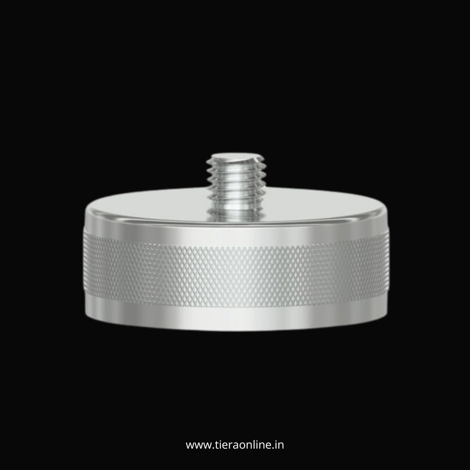
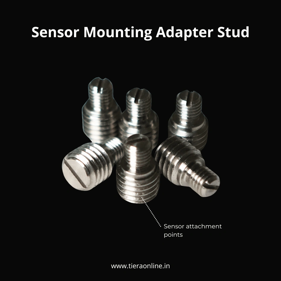 Sensor Mounting Adapter StudTM101-1A : TIERA SS304 Adapter Stud for sensor mounting₹260View →
 Magnetic Mounting Pad for Vibration sensorTMA-101-1A : SS 304 Magnetic Mount for Accelerometers and Vibration Sensors.₹800View →
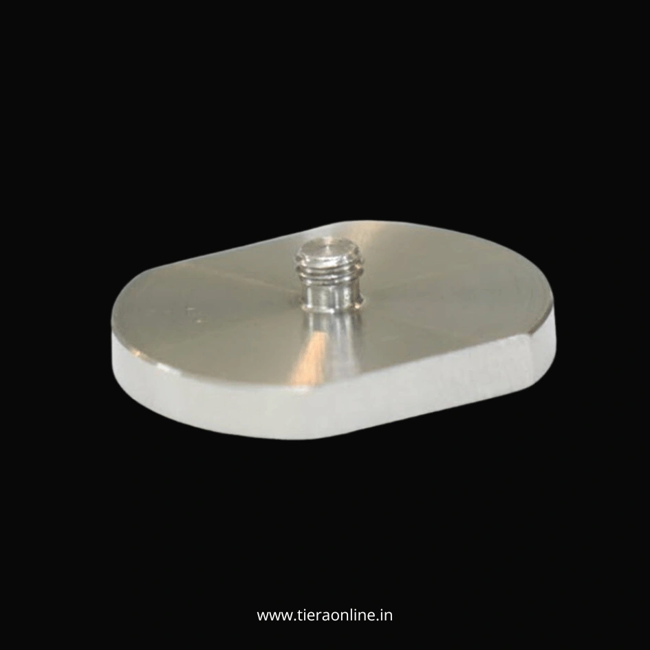 Cementing pad for Accelerometer mountingTAP-101-1-A : SS 304 Cementing pad for Accelerometers and Vibration sensors₹500View →
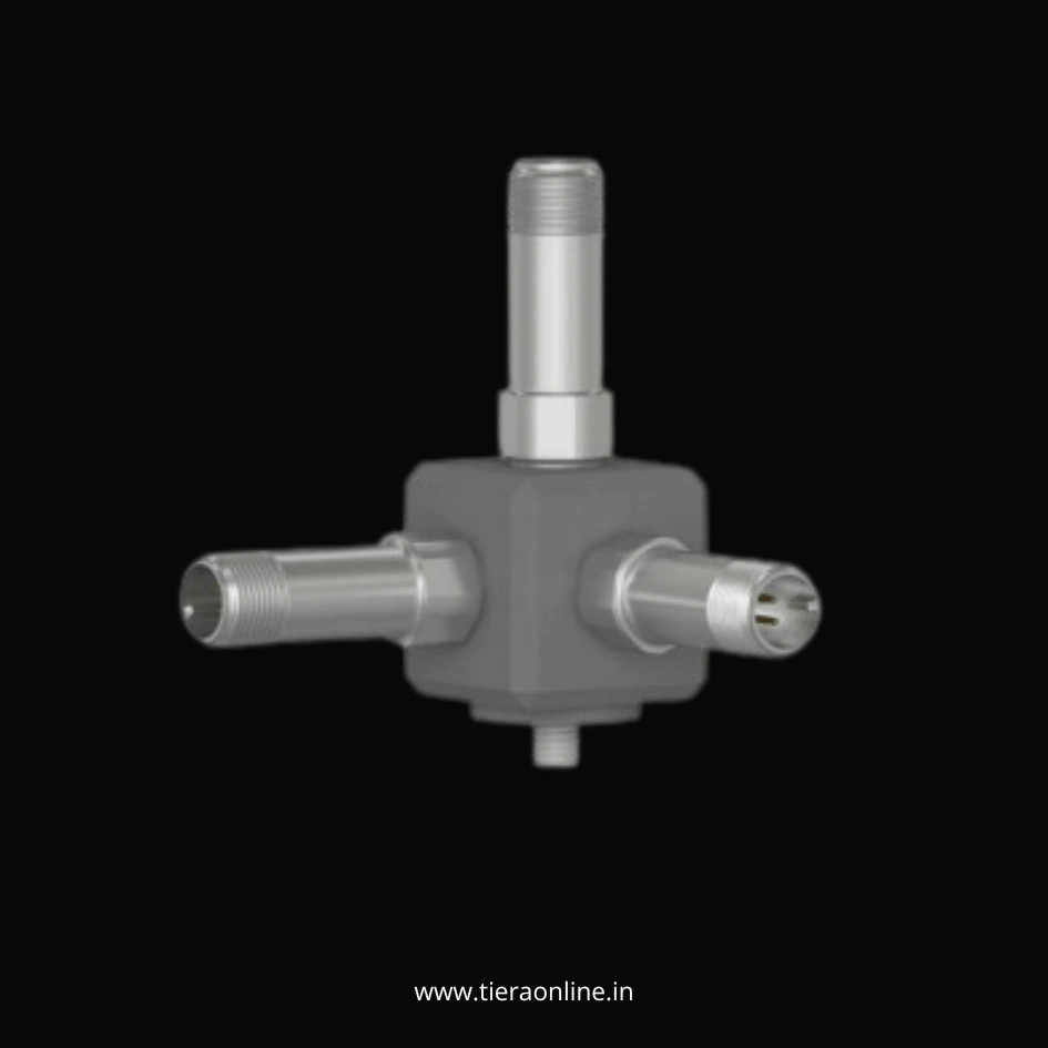 Triaxial Accelerometer Mounting BlockTMB-101-1-A : SS304 Triaxial Mount for Accelerometer Mounting Low Cost Customizable Allows attachment of 3 single axis accelerometers₹2,500View →
Use cases
Where this shows up in the field
The bandwidth you keep is decided by hardware that costs less than one missed bearing
TIERA stocks the unglamorous parts this post is about: an SS304 triaxial mounting block for permanent locations, a quick-release magnetic mount for route work, adhesive pad sets for non-magnetic or unmachinable surfaces, and low-noise and armored IEPE cables so the signal that survives the mount also survives the run back to the instrument. Every accessory carries its own datasheet in the public TIERA datasheets repository, including the mounted-configuration details this post says to check.
On the sensing side, the range runs from general-purpose and compact accelerometers to a dedicated low-frequency unit for slow machinery, feeding PhonoVibe 24-bit DAQ systems whose bandwidth reaches well past any mounting ceiling discussed here — so the mount, not the instrument, stays the only thing you need to think about.
- TMB-101-1-A SS304 triaxial mounting block for permanent, repeatable locations
- TMA-101-1 magnetic mount and TAP-101-1A adhesive pad set for route and non-magnetic surfaces
- Low-noise coaxial and armored accelerometer cables (CA-101 / CA-103, 5 m standard)
- Accelerometers from compact to low-frequency, plug-and-measure with PhonoVibe DAQs
Where this sits on the TIERA learning ladder.
The theory behind this article is covered free, in full, by the TIERA 101 primers: Accelerometer & DAQ Selection 101, Measurement Setup 101. They are self-paced, interactive, and end in an exam and a certificate.
TCAT adds examined, instructor-led depth on measurement setup — mounting choices, mounted-resonance checks, and defensible survey practice — with proctored exams that certify competence; the free primers explain, TCAT verifies.
TIERA 101 is a free introductory primer, not an accredited ISO certification, and its hours do not count towards the formal training ISO 18436 requires.