Published · Updated
What Makes a Good DAQ: Dynamic Range, Noise Floor, and How to Test One
Two DAQ units both say 24-bit. One shows the bearing defect three months before failure; the other buries it in its own noise. Drive a live DAQ bench that quantises, clips, aliases and adds noise to a real machine signal, then take away the bench tests you should demand before you buy.
The box between the sensor and the answer
An accelerometer does not produce a spectrum. It produces a small analogue voltage that is proportional to acceleration, riding on a DC bias, down a cable that is picking up whatever the plant is radiating. Everything between that voltage and the number you write in a report happens inside the data acquisition unit. If the DAQ is honest, the spectrum is a picture of the machine. If it is not, the spectrum is a picture of the DAQ, and no amount of analysis software will tell you which one you are looking at.
Six jobs happen inside the box. It supplies constant current to power the sensor's built-in amplifier and holds the bias voltage steady. It conditions the signal: blocks the DC bias, applies gain to match the sensor's output to the converter's input range. It filters, with an analogue low-pass ahead of the converter that removes everything above half the sampling rate. It samples, holding the voltage steady while the converter works. It digitises, turning volts into counts. And it timestamps, so that channel 3 and channel 7 are known to have been captured at the same instant and so that a tacho pulse can be tied to the exact sample it arrived on.
A cheap unit does all six of those things. It just does several of them badly, and the specific ways it does them badly are the subject of the rest of this post.
Bits are a promise. ENOB is the measurement.
- For an ideal converter, dynamic range is roughly 6.02 times the bit count plus 1.76 dB — about 98 dB at 16 bits and 146 dB at 24. No real instrument reaches the 24-bit figure.
- A measurement-grade front end of this class typically specifies 100 to 115 dB, roughly 16 to 19 effective bits; a weak one lands nearer 12. Both are 24-bit converters.
- Bit count alone is a weak predictor, because an FFT's processing gain lets a tone be seen below the broadband floor. What decides it is the analogue noise floor underneath.
Resolution is the number of steps the converter divides its input range into. A 24-bit converter has 2^24, about 16.8 million steps. Spread across a ±5 V range, one step is about 0.6 microvolts. That is the promise printed on the box.
Dynamic range is the ratio between the largest signal the channel can take without clipping and the smallest it can resolve above its own noise, and it is usually quoted in decibels. For an ideal converter with nothing but quantisation error, dynamic range is roughly 6.02 times the number of bits plus 1.76 dB: about 98 dB for 16 bits, about 146 dB for 24 bits. No real instrument achieves the 24-bit figure, because the amplifiers, references and power supplies in front of the converter add noise of their own.
That is what the effective number of bits, ENOB, measures. It is the resolution the channel actually delivers once real noise and distortion are included, worked back from the measured signal-to-noise-and-distortion ratio; the definition and the sine-wave test that produces it are set out in IEEE 1241, the standard for terminology and test methods for analogue-to-digital converters. Nobody reaches the ideal figure. A measurement-grade 24-bit front end of this class typically specifies somewhere between 100 and 115 dB of dynamic range, which is roughly 16 to 19 effective bits, while a weak front end can land nearer 12. Both are 24-bit converters. Only one of them is a 24-bit-class measurement, and the difference is not academic.
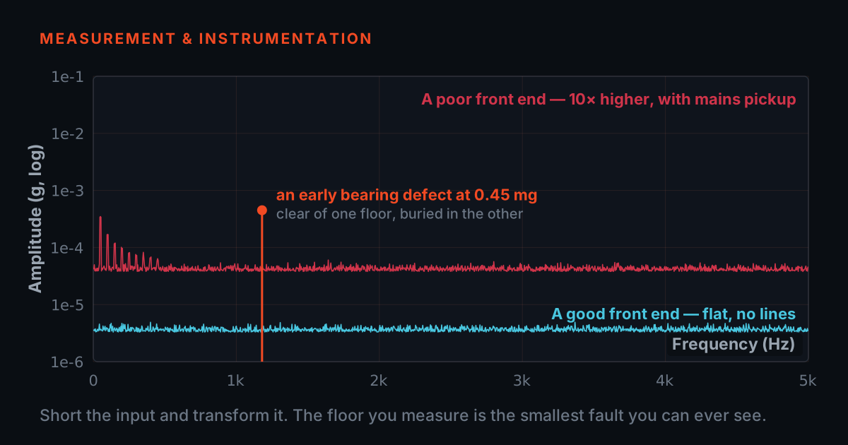
Here is why it decides diagnoses. Take a 1500 rpm fan with a moderate unbalance at 25 Hz and an early outer-race bearing defect. The unbalance peak is around 4 g. The bearing defect peak, in its first weeks, might be 4 milli-g — a thousand times smaller, 60 dB down. Both live in the same spectrum, taken through the same channel, with the range set by the largest peak. If the channel has 95 dB of usable range the defect clears the floor with margin. If it has 60 dB, the defect is at the floor, and whether it appears in your report is decided by luck.
One important qualification, because it is the part most articles get wrong. Narrowband analysis is not stuck with the broadband dynamic range. An FFT splits the broadband noise across all its lines while a genuine tone stays in one line, so a tone can be seen below the broadband noise floor by roughly ten times the logarithm of the ratio of the analysis bandwidth to the resolution bandwidth — about 25 dB for a 1024-point FFT over a 1280 Hz span. That processing gain is why a 16-bit instrument is not automatically useless. It also means bit count alone is a weak predictor of what you will see. What actually decides it is the analogue noise floor underneath, which no amount of FFT length can improve past the point where it stops being random.
The noise floor is the bottom of your spectrum
- Convert both instruments to the same form and bandwidth before comparing. Nanovolts per root hertz is the form that compares directly; a broadband microvolt figure only compares if the bandwidth and averaging happen to match.
- RMS averaging does not lower the true noise floor. It removes the scatter — the apparent floor falls 5 to 8 dB over the first handful of averages and then stops moving.
- The question is not is this DAQ quiet. It is whether its input noise density sits comfortably below your sensor's, at the frequency you care about and the range you will use.
The noise floor is the output the channel produces when the input is not moving. It comes from thermal noise in resistors, current and voltage noise in the input amplifier, ripple from the power supply, digital switching that leaks into the analogue section, and quantisation. It sets the smallest vibration you can trust, because anything below it is the instrument talking to itself.
It gets specified in three common forms, and they are not interchangeable. As a broadband figure — so many microvolts RMS over a stated bandwidth, which is meaningless unless the bandwidth is stated. As a spectral density — so many nanovolts per root hertz, which is bandwidth-independent and therefore the more useful number. Or as a relative figure in dBFS, decibels below full scale, which folds the range setting in with it. When you compare two units, convert both to the same form and the same bandwidth first, or you are comparing nothing.
Measuring it is straightforward and any supplier can do it: terminate the input properly — for an IEPE channel that usually means a resistive load that draws the constant current and presents the right impedance, not a bare short, because a short collapses the bias and the channel may not behave normally — then acquire with the same range, sample rate, window and averaging you use in service, and read the resulting spectrum. Averaging matters, and it matters in a way that is routinely misdescribed. RMS (magnitude) averaging — what an analyser normally means by 'linear averaging' of spectra — does not lower the true mean noise floor at all. What it removes is the scatter: a single-block noise floor is spiky, and its spikes sit several decibels above the mean, so the apparent floor falls by roughly 5 to 8 dB over the first handful of averages and then stops moving however many more you add. Vector (synchronous) averaging is the one that genuinely reduces incoherent noise, by the square root of the number of averages — 12 dB for sixteen. The practical consequence is the same either way: ask which kind of averaging was used and how many, because a supplier quoting a spiky single-block figure and one quoting a well-averaged one are not quoting the same measurement.
One practical consequence: the quantisation part of the floor scales with the input range. The step size is the range divided by 2 raised to the number of bits, so choosing ±10 V when your sensor never exceeds ±0.5 V throws away 26 dB for nothing. The analogue part of the floor does not scale that way — it is there whatever range you pick.
There is a criterion that turns all of this into a single question you can answer, and answering it honestly means starting from the sensor rather than from the brochure. The sensor has a noise floor of its own, and it is a function of frequency — a spectral-noise figure quoted without the frequency it applies at is not a number, it is a decoration. The CTC 100 mV/g standard-size accelerometers TIERA supplies publish 2 µg/√Hz at 1 kHz, which at 100 mV/g is 0.2 µV/√Hz — 200 nanovolts per root hertz — at the DAQ input. Lower down the band the same physics gives a larger number: the 50 mV/g parts in the same catalogue publish 8 µg/√Hz at 10 Hz falling to 2.5 at 100 Hz and 1.7 at 1 kHz, and the low-power parts built for battery-powered wireless nodes publish 60 µg/√Hz at 10 Hz. So there is no single 'sensor noise floor' to compare against — there is a curve, and a part number.
That is what makes the comparison uncomfortable, and worth doing. A measurement-grade 24-bit IEPE front end of this class typically specifies an input-referred noise density of the order of 100 nanovolts per root hertz on its most sensitive range. Against a good 100 mV/g piezo at 1 kHz that is roughly 200 nV/√Hz of sensor against roughly 100 nV/√Hz of instrument — about 6 dB of margin, not the two or three orders of magnitude the phrase 'the sensor always dominates' invites you to assume. Against the same sensor at 10 Hz, or against a noisy low-power MEMS part anywhere, the DAQ disappears into insignificance and the sensor is unambiguously the limit. Both situations are normal; which one you are in depends on the part and the frequency, and you cannot know without both numbers.
This is why the figure is worth having as a density: densities compare directly between two instruments, while broadband microvolt figures compare only if the bandwidth and the averaging happen to match. The DAQ's job is not to be perfect; it is to be quieter than the transducer at the frequencies that carry your diagnosis, so the measurement is limited by the sensor and not by the instrument reading it. So do not ask 'is this DAQ quiet?'. Ask 'is this DAQ's input noise density comfortably below my sensor's, at the frequency I care about and the range I will use?'. Ten times below is comfortable. Equal is a 3 dB penalty you paid for nothing. Above it, you bought a sensor whose performance you cannot reach.
The anti-alias filter has to be in the hardware
- The filter must be analogue and ahead of the converter. Once the folding is in the samples, no digital operation separates a folded component from a genuine one at the same frequency.
- The rejection has to be at least as large as the channel's usable dynamic range — an alias attenuated by 60 dB onto a floor 100 dB down means the filter, not the converter, now sets your working range.
- Test it yourself: feed a clean tone at 1.5 times Nyquist and look for a peak at the folded frequency. Repeat at two or three sample rates, because on some designs the filter follows the rate and on others it does not.
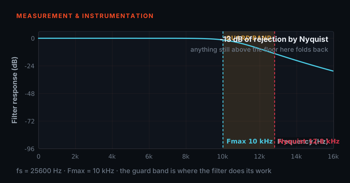
Any energy above half the sampling rate does not get rejected by the converter. It folds down and appears as a peak at a lower frequency, indistinguishable from a real one. It is not noise; it is a perfect impostor. The theory, the folding arithmetic and a playground to break it yourself are already covered in our post on sample rate, Fmax and anti-aliasing and the hands-on aliasing playground, so this post takes the theory as read and looks only at the hardware question.
The hardware question is where the filter sits. It must be analogue, and it must sit ahead of the converter, because once the folding has happened in the samples there is no digital operation that can separate the folded component from a genuine one at the same frequency. A modern instrument typically oversamples — runs the converter far faster than the output rate, uses a gentle analogue filter to protect that much higher Nyquist frequency, then does the sharp filtering digitally before decimating to the rate you asked for. That is a legitimate architecture and it is what most good units do. What is not legitimate is no analogue protection at all.
You can test for it without opening the box. Feed a clean sine from a generator at a frequency above the Nyquist of the rate you have selected — say 1.5 times Nyquist — at a decent amplitude, and look at the spectrum. On a properly filtered channel you should see nothing but floor. On an unprotected one a peak appears at the folded frequency, and its height tells you the rejection. Ask for the stopband rejection figure in decibels at the frequency you care about. There is a principle behind the number you should expect, rather than a number to memorise: the rejection has to be at least as large as the channel's usable dynamic range. An alias attenuated by only 60 dB, landing on a floor that is 100 dB down, means the filter and not the converter now sets your working range. In practice a measurement-grade unit of this class typically specifies 80 dB or better at Nyquist, and the digital decimation filters in oversampled sigma-delta designs are commonly quoted near 100 dB. Repeat the test at two or three sample rates, because on some designs the filter follows the rate and on others it does not.
The DAQ bench: break the measurement yourself
The simulator below runs one synthetic machine signal through a channel whose quality you control. The machine is a 1500 rpm fan: a large 4 g unbalance component at 25 Hz, a small second harmonic, an early outer-race bearing defect at 90 Hz at 4 milli-g with two harmonics, and a component at 1850 Hz that sits above the Nyquist frequency of the 2560 Hz sampling rate — think of a gear mesh, a drive switching frequency or a bearing resonance.
The sensor is a 100 mV/g accelerometer with a fixed self-noise of 0.2 microvolts per root hertz — 2 micro-g per root hertz at 1 kHz, the figure CTC publishes for the 100 mV/g standard-size units TIERA supplies — which is always present and which you cannot control. That is the floor the DAQ has to stay underneath, and note how low it is: at the default 100 nV/√Hz the instrument is only about 6 dB below the sensor, so it is already contributing a visible share of the floor before you touch anything. Four controls decide whether the fault survives: the converter's bit count, the DAQ's own input noise density, the input range you selected, and whether the anti-alias filter is present. Watch the readout that compares the DAQ's noise with the sensor's: it is the number that decides most of it.
Indicative signal model for teaching, not a measurement. Sampling 2560 Hz, 1024-point FFT, Hann window, one block. Sensor: 100 mV/g with a fixed 0.2 µV/√Hz self-noise — 2 µg/√Hz at 1 kHz, CTC's published figure for the 100 mV/g standard-size units, treated here as flat across the 0–1280 Hz band. That flat treatment is optimistic at the low end, where real piezo noise rises towards DC. The model also has no mechanical background: on a real machine broadband vibration, not sensor electronics, usually sets the floor a small bearing peak has to clear, so the margins here are the instrument's best case, not a route measurement. The DAQ noise density and the anti-alias filter's fixed 80 dB stopband rejection are class typicals for teaching, not specifications of any product. Quantisation, clipping and alias folding are computed on the synthesised waveform.
IEPE current, compliance voltage and the bias reading nobody checks
- Compliance voltage, not input range, is what squashes the top of large events — and widening the range will not fix it.
- That failure appears exactly when the measurement matters: impact tests, run-ups through resonance, a machine already in trouble.
- Cable capacitance and available drive current together cap the highest frequency the sensor can drive at a given amplitude, so long runs need the sensor maker's cable-length curve for your supply current.
An IEPE accelerometer — also called ICP or CCLD — contains a miniature amplifier that has to be powered. The DAQ supplies a constant current, typically 4 mA, down the same coaxial cable that carries the signal back. The sensor sits at a DC bias voltage, commonly 8 to 12 V, and the vibration signal swings above and below that bias. The DAQ blocks the DC and keeps the AC.
Compliance voltage is the highest voltage the current source can hold up while still delivering its rated current. If the supply's compliance is 18 V and the sensor's bias is 11 V, you have 7 V of swing available before the current source runs out of headroom, and the top of every large event gets squashed. This is why an under-specified supply fails exactly when the measurement matters: on impact tests, on run-ups through resonance, on a machine that is already in trouble. It looks like clipping, but the input range is not the cause and widening the range will not fix it.
Long cables cost you in a second way. The cable capacitance and the available drive current together set the highest frequency the sensor can drive at a given amplitude. With 4 mA, roughly 2 mA is available to drive the cable after the sensor's own bias current, and on a 100 metre run the high-frequency end of the response starts to distort at large amplitudes. If your cable runs are long, ask what current the supply provides and check the sensor manufacturer's cable-length curve for it.
The useful practical point: the bias voltage is a free sensor health check, and a DAQ that lets you read it is worth more than one that does not. A healthy channel reads a stable bias in the sensor's stated window. A bias near zero means a short in the cable or connector. A bias pinned near the supply rail means an open circuit — a broken conductor, a loose connector, or a dead sensor. Reading bias before a route takes seconds and saves you from trending a channel that was never connected. TIERA's 4-Channel IEPE Power Source carries a front-panel bias-voltage display for exactly this check.
Input range, overload, and what clipping does to a spectrum
Every input has a maximum voltage. Exceed it and the waveform flattens against the rail. The damage is worse than losing the peaks, because a flat-topped sine is mathematically a sine plus a series of harmonics. Clip a 25 Hz unbalance and the spectrum sprouts peaks at 50, 75, 100 and 125 Hz that were never on the machine. Those are the classic harmonic patterns of looseness and of a rubbing or misaligned coupling. An analyst who trusts the data diagnoses a fault that does not exist, and the strip-down finds nothing.
So overload indication matters, and there are two kinds. Some units flag only converter overload — the digital code hit its maximum. Others also flag analogue overload upstream, in the gain stage or the filter, which can saturate before the converter does and produce distortion without any full-scale code appearing. Ask which one the unit reports, and ask whether the overload flag is recorded with the data or only shown as a lamp on screen at the time. A flag saved in the file is what stops a bad measurement from silently entering a trend.
The opposite error is quieter and more common. Selecting a range far wider than the signal does not clip anything, so nothing warns you — but it throws away dynamic range in direct proportion. Going from ±0.5 V to ±10 V is a factor of 20, which is 26 dB of the margin your small bearing peak needed. Auto-ranging helps, but on machinery with intermittent impacts it can also chase transients and change the scaling mid-measurement, so know which behaviour your unit has before you trend anything.
Simultaneous sampling, and the degrees you lose to skew
- For an overall level reading, skew is harmless. For anything involving phase it is decisive, because a fixed time delay becomes a frequency-dependent phase error.
- You can estimate a multiplexed unit's skew yourself: it is about one sample period of the shared converter, so a 200 kS/s converter across eight channels puts roughly 5 µs between neighbours.
- Simultaneous with no phase-accuracy figure in degrees at a stated frequency attached to it is a marketing word.
Multi-channel DAQs come in two architectures. A simultaneous unit gives every channel its own sample-and-hold, or its own converter, so all channels freeze at the same instant. A multiplexed unit has one converter shared between channels by a switch, so channel 2 is sampled a little after channel 1, channel 3 a little after that. The delay between channels is called inter-channel skew.
For an overall level reading, skew is harmless. For anything involving phase it is decisive, because a fixed time delay becomes a frequency-dependent phase error: the error in degrees is 360 times the frequency times the skew. Fifty microseconds of skew is 0.45 degrees at 25 Hz — negligible. The same 50 microseconds is 18 degrees at 1 kHz and 36 degrees at 2 kHz. Balancing at 25 Hz survives it. A gearbox transfer-path measurement at 1 kHz does not, and a mode shape assembled from channels with unknown relative phase is not a mode shape.
Balancing is where this becomes money. The correction weight is placed at an angle derived from the measured phase. If the measured phase is wrong by an angle, the weight goes on at the wrong angle, and the residual unbalance after a perfect single-shot correction is at least twice the original amount times the sine of half the phase error. Ten degrees of phase error leaves about 17 percent of the original unbalance behind no matter how good your influence coefficients are. Twenty degrees leaves about 35 percent. That is a second trip to site, and then a third.
Two things to ask, and they are different questions. First: is the sampling truly simultaneous, or multiplexed? For a multiplexed unit you can estimate the skew yourself without asking anyone, because it is about one sample period of the shared converter: a 200 kS/s converter switched across eight channels puts roughly 5 microseconds between adjacent channels, which is 1.8 degrees at 1 kHz and 18 degrees at 10 kHz. Second: what is the specified inter-channel phase accuracy, in degrees, at a stated frequency? For a simultaneous-sampling instrument of this class the typical published figure is around a tenth of a degree at 1 kHz and under a degree at the top of the band, because when the converters share one clock the only error left is component tolerance in the analogue filters. 'Simultaneous' with no phase-accuracy number attached to it is a marketing word.
Indicative and illustrative. The phase error is the exact arithmetic for a fixed time skew; the residual figure assumes the phase error is the only error in an otherwise perfect single-shot correction, which is optimistic in the field.
Crosstalk, distortion, gain accuracy and drift
Crosstalk is signal from one channel appearing on another. It happens through shared grounds, capacitance between adjacent traces or connectors, and shared multiplexers. It is specified in decibels: a channel with -100 dB crosstalk shows a component from its neighbour at one hundred-thousandth of the amplitude. That sounds like nothing until you remember the numbers from earlier. A 4 g unbalance on channel 1, crosstalking at -60 dB, appears as 4 milli-g on channel 2 — the same size as the early bearing defect you were looking for. On a machine where all three axes see the same big 1x, weak crosstalk produces plausible-looking peaks at 1x on every channel, and you will spend a day chasing them. A measurement-grade multi-channel instrument of this class typically specifies -100 dB or better between channels at 1 kHz. The figure normally degrades as frequency rises, so a single number with no frequency attached to it is not a specification.
Total harmonic distortion is the fraction of the output that consists of harmonics the input did not contain, generated by non-linearity in the amplifiers and the converter. It matters for the same reason clipping matters: it fabricates harmonic families. It is defined and measured alongside ENOB and SINAD by the same IEEE 1241 method, and for this class of instrument a typical published figure is -90 dB or better across the working band, stated at an amplitude near full scale — distortion always rises as you approach the rails, so the amplitude the figure was measured at is part of the figure.
Gain accuracy is how close the reported amplitude is to the true amplitude, usually quoted as a percentage of reading at a stated frequency. It is what makes your 4.1 mm/s comparable with the reading someone else took last quarter on a different unit. Drift is how much that gain and the DC offset move with temperature and with time since power-on. Typical published figures for this class of instrument run from ±0.1% to ±0.5% of reading at a stated frequency, with temperature coefficients in the tens of parts per million per degree Celsius. A specification written as 'gain accuracy ±0.5% at 1 kHz, temperature coefficient 50 ppm per degree C' tells you something. 'High accuracy' tells you nothing.
Drift also has a practical face: warm-up. Many instruments need ten to thirty minutes at operating temperature before their gain and offset settle. If your route starts with the DAQ cold out of a van in January and ends three hours later, the first readings and the last readings were taken on subtly different instruments. Ask for the warm-up time and the drift over it, then build it into the route.
Timing: sample clock accuracy, jitter and the tacho input
The sample clock sets the frequency axis. If the clock is 0.1 percent fast, every frequency you read is 0.1 percent high — at 1x on a 1500 rpm machine that is 0.025 Hz, invisible; at a 30 kHz gear-mesh harmonic it is 30 Hz, enough to shift a sideband family off the cursor you set last month. Clock accuracy is specified in parts per million. A plain crystal oscillator of the kind used in this class of instrument is typically ±25 to ±50 ppm, and designs built around a temperature-compensated oscillator typically publish a few ppm. Anything in the tens of ppm is fine for machinery work.
Jitter is the random variation in when each sample is actually taken. Its effect grows with frequency and with signal amplitude: a large high-frequency component sampled with jitter smears into a raised noise skirt around its own peak. In practice, jitter is what stops you seeing a small sideband sitting close to a big gear-mesh line. It is specified in picoseconds RMS, with typical published figures for measurement instruments of this class running from tens to a few hundred picoseconds, and it is one of the specifications a cheap unit is least likely to publish at all.
A tacho or trigger input is a separate matter and it is not optional for two jobs. Order tracking on a variable-speed machine needs the shaft position tied to the samples, so that a spectrum can be computed against shaft orders instead of hertz — the reason and the method are in the order-tracking explainer. Phase measurement for balancing needs the same reference, because phase is meaningless without something to be relative to. When you evaluate a unit, ask whether the tacho is sampled on the same clock as the analogue channels or handled separately, and what its timing uncertainty is, because that uncertainty lands directly on your phase reading and feeds straight into the skew arithmetic in the simulator above.
How to test a DAQ: the bench tests to demand
None of the above requires you to take anyone's word. Every one of these tests can be run with a signal generator, a calibrated reference, a resistor and an afternoon. The methods are not improvised either: IEEE 1241 sets out the terminology and test methods for analogue-to-digital converters, IEEE 1057 does the same for digitising waveform recorders, and ISO 16063-21 covers calibration of a vibration transducer by comparison against a reference, which is what test 2 becomes once you include the sensor. Ask any supplier — including us — to send you the results for the exact model and configuration you are buying, measured at the settings you will actually use. A supplier who can produce these numbers has measured their own product. A supplier who cannot has told you something too.
1. Shorted or terminated input noise floor. Terminate every input with the correct load for the input type, acquire at your working sample rate and range, apply the window and number of averages you use in service, and record the spectrum. Ask for the floor in nanovolts per root hertz, and separately in dBFS at a stated range. Ask for the number of averages used, because that number alone moves the answer by 10 dB or more. Repeat at the widest and narrowest input range: the floor should scale with range if quantisation dominates and stay flat if the analogue front end dominates, and which of the two you see tells you where the noise is coming from.
2. Amplitude and frequency accuracy against a reference. Feed a precise sine of known amplitude and frequency and compare what the DAQ reports. Do it at several amplitudes across the range and at several frequencies across the band, because gain error is rarely constant across either. The reference can be a calibrated signal generator for the electrical path, or a calibrated shaker and reference accelerometer if you want to verify the whole chain including the sensor. Ask for the error as a percentage of reading, with the reference and its calibration state named.
3. Anti-alias rejection. Feed a clean tone above Nyquist — 1.5 times Nyquist is a good choice, and repeat just above Nyquist where filters are weakest — at a large amplitude, and measure the height of whatever appears at the folded frequency. Ask for the rejection in decibels at Nyquist and at 1.5 times Nyquist, and ask whether the filter tracks the sample rate. Then repeat the test yourself on the unit at your two most-used sample rates.
4. Crosstalk. Drive one channel with a large tone, terminate all the others properly, and measure the level of that tone on each of them. Ask for the worst-case channel-to-channel figure in decibels, at a stated frequency, with adjacent channels identified — crosstalk is usually worst between physical neighbours. Also ask whether the figure was measured with the other channels terminated or left open, since open inputs flatter the result.
5. Inter-channel phase and gain match. Split one generator output to every channel through equal-length cables and acquire them all. The signals are identical by construction, so any difference in reported amplitude is gain mismatch and any difference in reported phase is skew plus filter mismatch. Ask for phase match in degrees at a stated frequency, and repeat the measurement at the top of your working band, not just at 100 Hz.
6. Overload and recovery. Drive an input past full scale, then bring it back down, and watch how long the channel takes to return to a correct reading. Some designs recover in microseconds; some take milliseconds and blur a whole block of samples. Ask whether the overload is flagged, whether the flag distinguishes analogue from converter overload, and whether it is saved with the data.
7. Warm-up and drift. Power the unit from cold and record a terminated-input reading and a known-tone reading every minute for an hour. Ask for the time to reach the stated accuracy, and for gain and offset drift in ppm per degree C. This is the test people skip, and it is the one that explains why last winter's trend has a step in it.
8. IEPE supply under load. Check that the constant current is what it claims with a real sensor connected, that the bias voltage sits where the sensor expects, and that compliance holds up with your longest cable at your largest expected amplitude. The failure this catches — distortion only on large signals, only on long runs — is otherwise almost impossible to diagnose in the field.
One caution on reading results: a specification measured at 1 kHz with 200 averages at the narrowest range on a bench at 23 degrees C is a real number, and it is not the number you will get at 20 kHz with 4 averages at the widest range in a plant. Ask for conditions with every figure. The conditions are the specification.
A second caution, on the typical figures quoted throughout this post. Every one of them describes a class of instrument — what a measurement-grade unit of this type is normally specified to achieve, and where that expectation comes from. None of them is a specification of any particular model, TIERA's included. Use them to know what to ask for, and to recognise an evasive answer when you get one. Then get the real numbers, for the real unit, under your conditions, in writing.
What the cheap unit actually costs
- Four countable costs, all of which land on the maintenance budget rather than the capital one: false alarms, missed early faults, unrepeatable trends, and balancing jobs that will not converge.
- The early stage a CM programme exists to catch is exactly the stage where the defect sits 50 or 60 dB below the running-speed peak. A channel that cannot see 60 dB down does not shorten the warning — it removes it.
- DAQ quality does not buy you a nicer spectrum. It buys you the right to believe the spectrum.
The argument for spending more is not about brand and it is not about feeling better. It is about four specific, countable costs that land on the maintenance budget rather than the capital budget.
False alarms. A high noise floor and poor crosstalk produce peaks that are not on the machine. Every one of them is a work order, an inspection, sometimes a strip-down that finds nothing. Three of those a year on a plant of any size costs more than the price difference between a good DAQ and a poor one, and the second-order cost is worse: once the analysts have chased three ghosts, they stop believing the next real indication.
Missed early faults. This is the expensive one. The whole economic case for condition monitoring is catching a bearing at the stage where it is a planned overnight replacement instead of an unplanned three-day outage with collateral damage to the shaft and the seals. That early stage is exactly the stage where the defect signal is 50 or 60 dB below the running-speed peak. A channel that cannot see 60 dB down does not shorten the warning; it removes it.
Unrepeatable trends. Gain drift, warm-up drift and auto-ranging that changes scale mid-route produce a trend that moves for instrument reasons. You cannot set an alarm level on a trend like that, so you either set it so wide it never triggers or so tight it always does. Either way the programme stops working, and the usual conclusion drawn is that condition monitoring does not work here.
Balancing jobs that will not converge. The phase simulator above puts a number on it. A phase error you cannot see leaves a residual you cannot remove, so you go back, take another set of readings, add another trial weight, and go back again. Two extra site visits on one machine will typically cost more than the difference in instrument price, and the customer watching you do it draws their own conclusion.
The honest summary is that DAQ quality does not buy you a nicer spectrum. It buys you the right to believe the spectrum. Everything downstream — the analysis software, the alarm bands, the AI model, the analyst's judgement — is built on the assumption that the numbers are the machine. That assumption is either true or it is not, and it is decided in the box.
Where to learn this properly
If the terms in this post were new, the free TIERA 101 primers at 101.tieraonline.in cover the ground in order: Accelerometer & DAQ Selection 101 works through the sensor and the acquisition chain, and Measurement Setup 101 covers ranges, rates, mounting and building a route that repeats. They are free primers, not accredited certification.
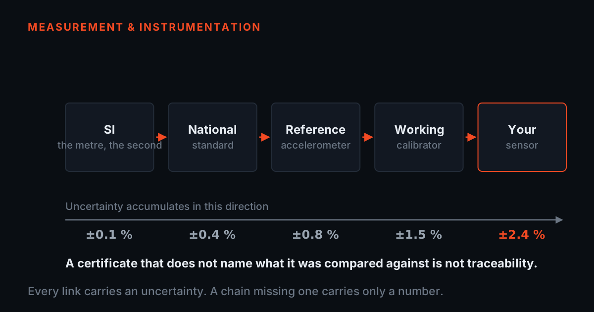
Two neighbouring posts finish the picture. The sampling theorem, Fmax and line selection are in sample rate, Fmax and anti-aliasing, with a hands-on version in the aliasing playground. What makes an amplitude number traceable rather than merely precise is in calibration and traceability. And when you are ready for formal, examined credentials, the TCAT analyst programme on our services page (/services) runs proctored examinations at exams.tieraonline.in.
TIERA instruments that do this work.

PhonoVibe Series — Sound & Vibration DAQ
TIERA's own USB DAQ line for this job — 24-bit converters, simultaneous sampling on every input, and IEPE power on every channel, in 2, 4, 8 and 16-channel models.
- ADC resolution
- 24-bit across the series
- Channels
- 2 / 4 / 8 / 16 (D, Q, O, HD)
- Sampling & bandwidth
- 128 kHz per channel, 0.5 Hz – 60 kHz (Q, O, HD); 48 kHz, 2 Hz – 20 kHz (D)
- Sampling mode
- Simultaneous sampling on every input
- Sensor power
- 24 V, 4 mA constant current (IEPE/ICP/CCLD), TEDS supported
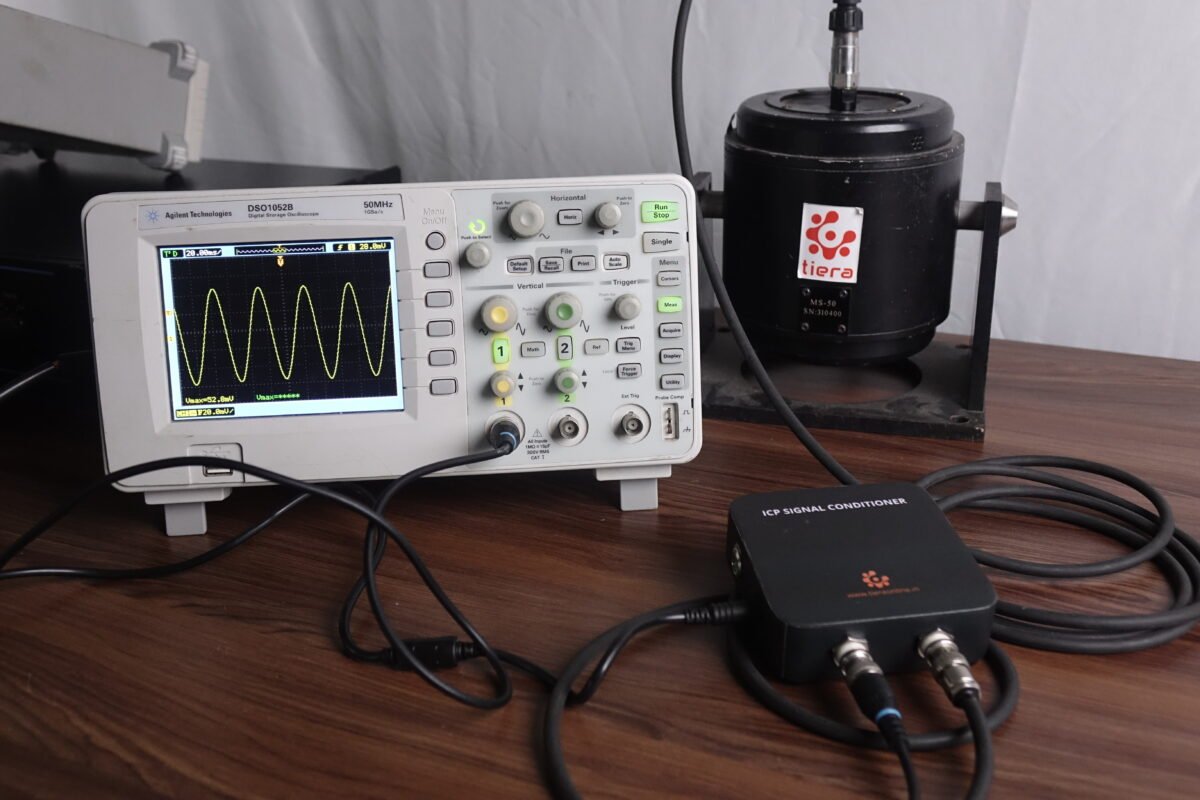
TSP Series IEPE Signal Conditioners
When the sensor excitation has to come from somewhere other than the DAQ — a third-party recorder, an oscilloscope, a DAQ without IEPE — this supplies the constant current at unity gain so the power source does not set your noise floor.
- Input type
- ICP® / IEPE
- Excitation
- 24 VDC, 4 mA constant current
- Gain
- 1 (unity) — no amplitude scaling
- Frequency response
- 0.5 Hz – 50,000 Hz
- Configurations
- TSP 02 single-channel, TSP 04 four-channel; BNC in / BNC out
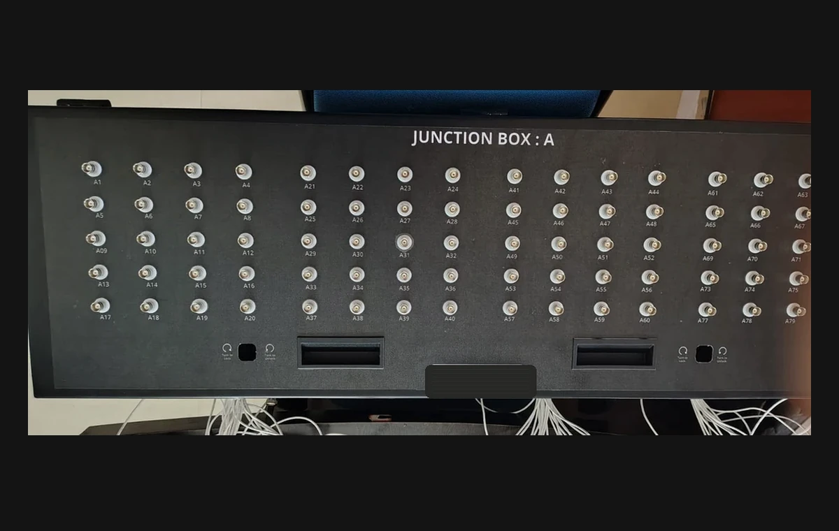
Custom High-Channel Junction Boxes
On a large array, the routing between the sensors and the DAQ is where crosstalk and cable damage are decided — these are built to a channel map, and delivered with a test report.
- Configuration
- Custom N-channel BNC (64, 80 and other layouts built to requirement)
- Routing
- Zone-based channel grouping with a clear channel map
- Chassis
- Lockable powder-coated, with cable glands
- Delivered with
- Test report for THD, noise floor and frequency response

T-Calibro Vibration Calibration System
Testing the DAQ only tells you about the DAQ. This closes the other end of the chain by checking accelerometer sensitivity back-to-back against a traceable reference.
- Method
- Back-to-back comparison calibration
- Reference frequency
- 159.2 Hz (≈1000 rad/s), per ISO 16063 back-to-back convention
- Compatibility
- All IEPE/ICP accelerometers
- Records
- T-Calibro software: automated calibration record and certificate generation
- Supplied with
- Factory calibration certificate
From the TIERA store
The kit for this job
What we would actually put in front of someone doing the measurement this post describes — not the whole catalogue.
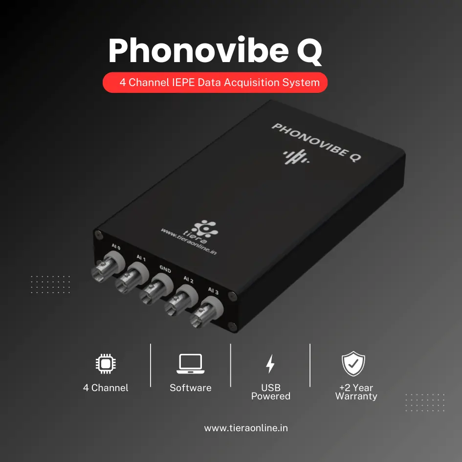 4 Channel IEPE Data Acquisition System – Phonovibe QFour Channels Standard plug & play USB Powered Take data from accelerometers, microphones, hammers, or any other IEPE Sensors T- VIB Software to acquire time waveforms, frequency spectra, overall vibration levels, FRF’s and octave measurements ** Windows 10 or above Operating System ** T-VIB Software base version comes with Time and Spectrum with Post processor TSAP 201. Check out TVIB Software regarding more module options.₹2,88,000View →
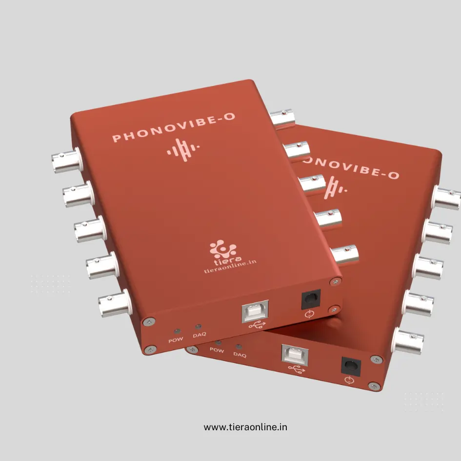 Phonovibe O- 8 Channel IEPE Data Acquisition SystemEight Channels Standard plug & play USB Powered Take data from accelerometers, microphones, hammers, or any other IEPE Sensors T- VIB Software to acquire time waveforms, frequency spectra, overall vibration levels, FRF’s and octave measurements ** Windows 10 or above Operating System ** T-VIB Software base version comes with Time and Spectrum with Post processor TSAP 201. Check out TVIB Software regarding more module options.₹4,60,800View →
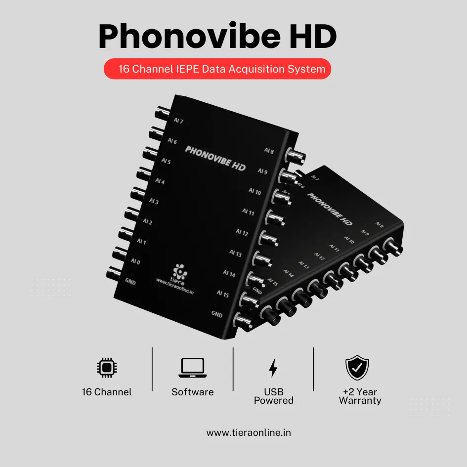 16 Channel IEPE Data Acquisition System-Phonovibe HDSixteen-Channel Data Acquisition System Plug & Play USB Powered Compatible with accelerometers, microphones, hammers, and other IEPE sensors T-VIB Software for time waveforms, frequency spectra, vibration levels, FRFs, and octave measurements Base version includes Time and Spectrum with TSAP 201 post-processor Explore additional modules with T-VIB Software₹7,20,000View →
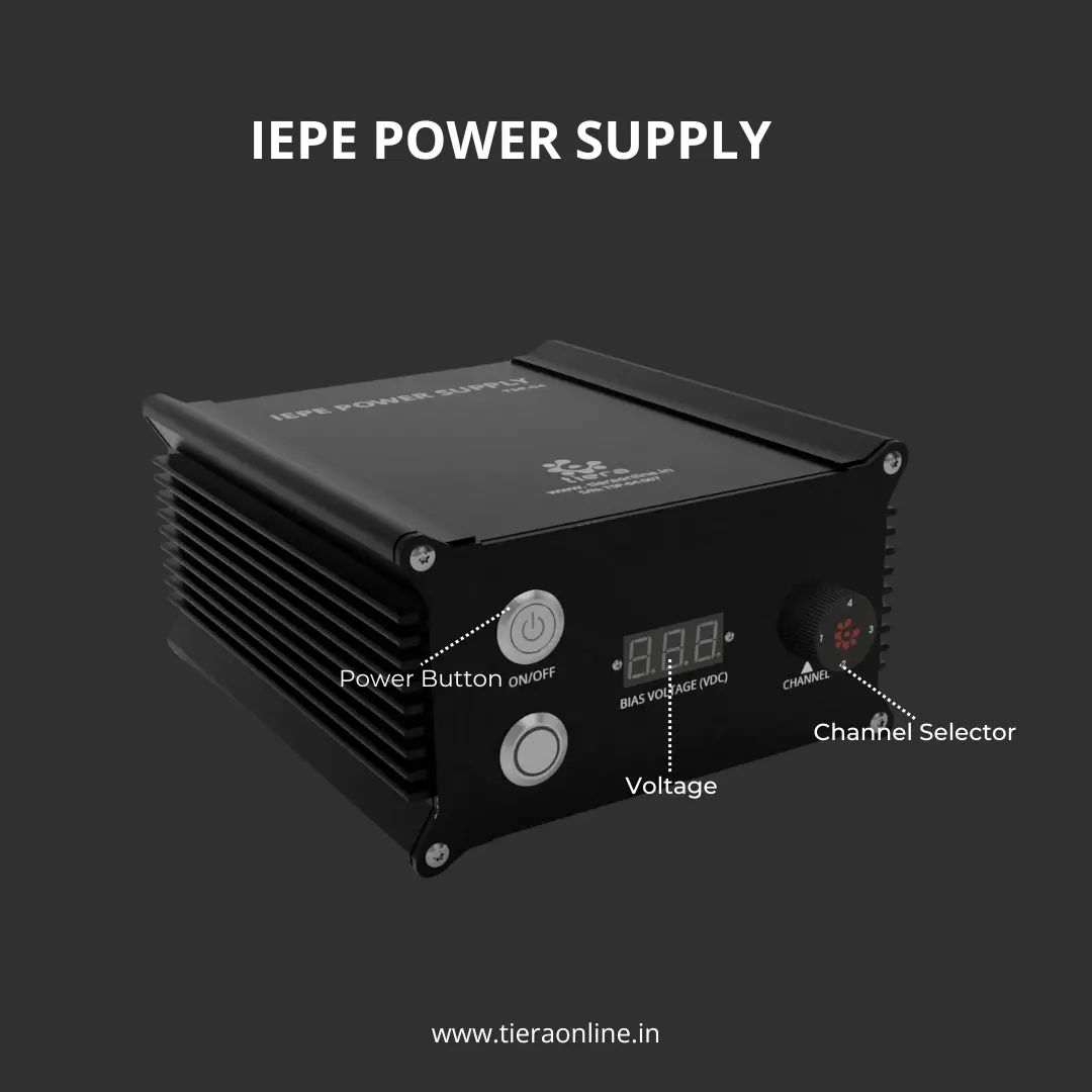 Four Channel IEPE Power Source-TSP 04Low Cost Customizable Connect ICP/IEPE Sensors to the oscilloscope or Voltage Input DAQ₹54,000View →
Use cases
Where this shows up in the field
Ask us for the numbers, then ask everyone else for the same ones
The tests in this post are the tests we think a buyer should run before spending money on any acquisition hardware, ours included. If you are evaluating a PhonoVibe against something else, send us the list — the noise floor at your range and averaging, the anti-alias rejection at your sample rate, the inter-channel phase match at your working frequency — and ask the other supplier for exactly the same list under exactly the same conditions. Comparing two sets of numbers measured under stated conditions is the only comparison that means anything.
If you would rather start from the job than the specification, tell us what you are measuring: how many channels, what frequencies, whether you need phase, whether the machine changes speed. That determines the channel count, the bandwidth and whether you need a tacho, and it usually rules out most of the catalogue in one conversation.
- PhonoVibe D / Q / O / HD — 24-bit USB DAQ, simultaneous sampling, IEPE power on every channel, TEDS, factory calibration certificate with 1-year validity
- TSP 02 / TSP 04 IEPE conditioners — unity-gain constant-current supply when the excitation has to sit outside the DAQ
- Custom N-channel junction boxes, built to your channel map and delivered with a test report
- T-Calibro — back-to-back accelerometer calibration so the other end of the chain is verified too
Where this sits on the TIERA learning ladder.
The theory behind this article is covered free, in full, by the TIERA 101 primers: Accelerometer & DAQ Selection 101, Measurement Setup 101. They are self-paced, interactive, and end in an exam and a certificate.
The free 101 primers cover the acquisition chain and how to set a measurement up so it repeats; TCAT Cat I-IV adds structured analyst training with proctored examinations at exams.tieraonline.in — a TIERA credential, not an accredited ISO certification.
TIERA 101 is a free introductory primer, not an accredited ISO certification, and its hours do not count towards the formal training ISO 18436 requires.