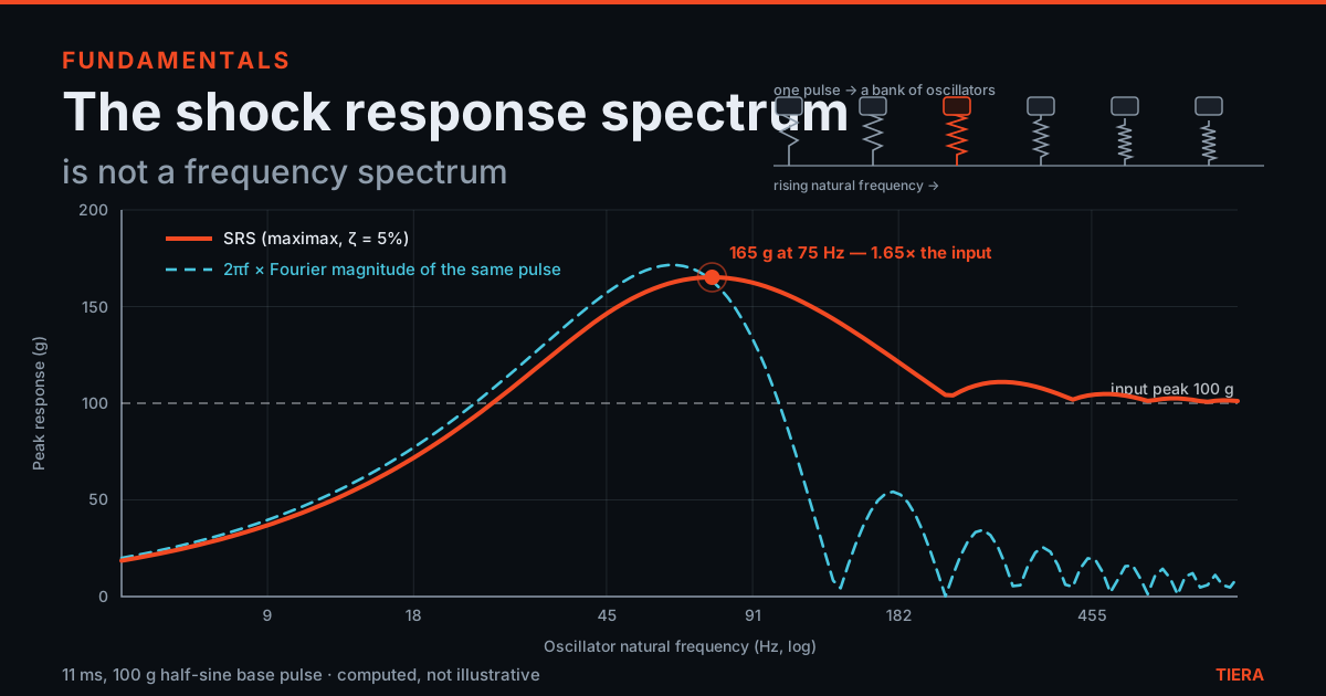
The Shock Response Spectrum Is Not a Frequency Spectrum
An SRS looks like a spectrum and is plotted like a spectrum, but it is not a decomposition of the pulse into frequencies — it is the worst thing a bank of imaginary oscillators ever felt. Build one live from a pulse you choose, watch the pulse's own Fourier magnitude diverge from it on the same axis, and compute a drop-shock level from height and pulse width.
It is plotted like a spectrum. It is not one.
- The whole, unaltered pulse is fed to a bank of imaginary single-degree-of-freedom oscillators, and each one reports exactly one number: the largest response it ever reached.
- The horizontal axis is that oscillator's natural frequency — a property of a hypothetical structure you might bolt on, not a frequency present in the pulse.
- Fourier answers what the pulse is made of. The SRS answers how badly it would hurt a structure that rings at f. Only the second is a damage question.
Almost every curve an engineer calls a spectrum is a decomposition. An FFT of a steady vibration signal splits it into sine waves: add the lines back up, with their phases, and you get the original waveform. Nothing is created, nothing is lost, and the height of a line is that ingredient's share of the whole. A shock response spectrum breaks that habit completely, and the fact that it is drawn on the same kind of log-log axes is responsible for most of the confusion around it.
An SRS is not built by taking a pulse apart. It is built by feeding the pulse — the entire pulse, unaltered — to a whole bank of imaginary single-degree-of-freedom oscillators, one after another, each with a different natural frequency. Each oscillator is shaken by the same base motion, rings in its own way, and reports exactly one number: the largest response it ever reached. Plot that number against that oscillator's natural frequency and you have the SRS. The horizontal axis is not a frequency present in the pulse. It is a property of a hypothetical structure you might bolt to the thing being shocked.
So the two curves answer two different questions. The Fourier magnitude answers what sinusoids the pulse is made of. The SRS answers how badly the pulse would hurt a structure whose natural frequency is f. Those are not the same question, they do not have the same answer, and this post exists to let you watch them come apart on one set of axes.
What the bank actually computes
Each oscillator in the bank is a mass on a spring and a dashpot, and the shock arrives as a motion of its base rather than as a force on its mass. Writing z for the mass's displacement relative to its base, x for its absolute displacement and y for the base's, the equation of motion is the ordinary damped SDOF one with the base acceleration as the forcing term: z'' + 2 zeta wn z' + wn^2 z = -y'', where wn = 2 pi fn is the undamped natural angular frequency and zeta is the fraction of critical damping. The quantity almost always plotted is the mass's absolute acceleration, x'' = -(2 zeta wn z' + wn^2 z), because that is what an accelerometer bolted to the mass would read.
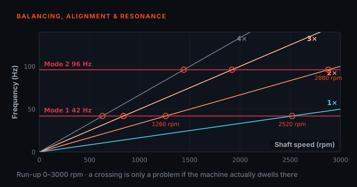
There is nothing exotic in that equation — it is the same forced SDOF system behind a Campbell diagram or a bump test, and TIERA's Endevco-era source for the classical treatment is Endevco TP219-1, "Basic Shock and Vibration Theory". What makes it a shock problem rather than a vibration problem is that the forcing is a transient: it starts, it ends, and afterwards the oscillator is left ringing down on its own with whatever energy it kept.
The simulator below integrates that equation for 110 oscillators, spanning natural frequencies from 0.05/T to 20/T where T is the pulse duration, using Smallwood's ramp-invariant recursive digital filter — a two-pole IIR form whose coefficients are derived by solving the SDOF response exactly for an input that varies linearly between samples. The step is adaptive, dt = min(T/400, 1/(30 fn)), so the fastest oscillator in the bank is still sampled thirty times per cycle and the peak is not missed between samples; each oscillator is run for the pulse duration plus two of its own periods, which is long enough for the after-the-pulse maximum to occur. A complete 110-point sweep costs a few milliseconds, which is why the curve redraws while you are still dragging the slider. The exact numbers for the settings you choose are printed under the plot.
Drive it: the SRS and the Fourier magnitude of the same pulse
Pick a pulse shape, set its duration and set the damping of the oscillator bank. The orange curve is the maximax SRS. The dashed cyan curve is the pulse's own Fourier magnitude, scaled by 2 pi f so that it carries the same units and can share the axis — that scaling is not a cosmetic fudge, and the section below on what the Fourier magnitude actually answers explains exactly what it means. The split toggle separates the SRS into its primary and residual halves. Hover anywhere on the plot to read all four curves at that natural frequency.
Three things are worth doing before you read on. With the half-sine selected, look at the far right of the plot: the SRS has settled onto the input peak of 100 g while the cyan Fourier curve has collapsed to a small fraction of it and is still falling — a stiff structure simply rides the base and feels what the base felt, no matter how little Fourier content sits at its natural frequency. Then switch to the square pulse and notice the SRS settles at roughly twice the input instead, because a perfectly vertical rise is a step and a step overshoots. Finally, drag the damping to zero and watch the residual curve fall exactly onto the Fourier curve — that is not a coincidence, it is the one place the two definitions genuinely coincide.
Primary, residual, maximax
- Primary is the largest response reached while the pulse is still on; residual is the largest reached after it ends; maximax is the larger of the two, and it is what a specification means when it says SRS with no further qualification.
- The soft end is residual-dominated — the pulse acts as an impulse, hands over a velocity change, and everything happens afterwards. The stiff end is primary-dominated. Amplification is largest where they cross.
- Positive and negative SRS are a further split real software makes and this page does not; any report should say which convention it used.
An oscillator is doing two different things over the course of a shock. While the pulse is still pushing on its base it is being driven; once the pulse stops it is ringing down on its own. Splitting the maximum by those two windows gives the two halves of the SRS. The primary spectrum is the largest response reached while the pulse is still on. The residual spectrum is the largest reached after it has ended. The maximax is simply the larger of the two, and it is what almost every test specification means when it says SRS with no further qualification.
The split is not bookkeeping. Which half wins tells you what kind of damage mechanism you are looking at. On the soft, low-frequency side of the bank the oscillator has barely started to move by the time the pulse is over — the pulse acts as an impulse, hands the base a velocity change, and everything interesting happens afterwards, so the residual dominates. On the stiff, high-frequency side the oscillator tracks the base almost exactly, reaches its maximum during the pulse and has almost no energy left over, so the primary dominates and the residual collapses. Somewhere in between they cross, and that crossing region is where the amplification is largest.
There is a further split that real analysis software makes and this simulator deliberately does not: positive and negative SRS, the largest excursion in each direction taken separately. It matters when a pulse is strongly asymmetric, because a structure can be far weaker in one direction than the other. Everything on this page uses the magnitude of the largest excursion in either direction, which is the maximax convention, and any real report should say which convention it used.
The Fourier magnitude answers a different question
- At zero damping the residual response equals 2πfn times the pulse's Fourier magnitude at fn — the one place the two definitions genuinely coincide.
- The Fourier magnitude describes only the ringing left over afterwards, for a structure with no damping at all. It says nothing about what happened during the pulse.
- A structure stiff enough to ride the base does not care that the pulse contains little energy at its natural frequency. It gets dragged along and feels what the base felt.
The two curves are not unrelated — and the relationship is exactly the reason so many people conflate them. Take the damping to zero. An undamped oscillator that has been kicked by a transient rings forever at its natural frequency, and the amplitude it settles into is set by precisely one thing: how much of the pulse's Fourier content sits at that frequency. Written out, the undamped residual acceleration response equals 2 pi fn times the magnitude of the pulse's Fourier transform evaluated at fn. That is the identity you can watch on the plot: drag damping to 0% and the green residual curve and the cyan Fourier curve become the same curve.
Which is the whole point. The Fourier magnitude describes the ringing that is left over — the steady state after the event, for a structure with no damping at all. It says nothing about what happened during the pulse, and nothing about what damping does. The maximax SRS includes both, which is why it stays stubbornly above the Fourier curve at the stiff end where the Fourier content has all but vanished. Set a half-sine and read the far right of the plot: the SRS is sitting on the input peak while the Fourier curve has fallen well over an order of magnitude below it and is still dropping — the readout under the plot prints both numbers. A structure stiff enough to ride the base does not care that the pulse contains little energy at its natural frequency. It gets dragged along and feels what the base felt.
The nulls make the same point from the other direction. A half-sine pulse's Fourier magnitude goes exactly to zero at a series of frequencies — you can see the cyan curve dive to the axis floor at fn·T = 1.5, 2.5, 3.5 and so on. A square pulse's goes to zero at every integer fn·T. If the SRS were a decomposition, those frequencies would be immune, and an SRS curve would have to dive with it. It does not. Nothing in the orange curve marks those frequencies at all, because the maximax at those points is set by the response during the pulse, and the during-the-pulse response is not a Fourier statement.
Two curves, two questions. "What is this pulse made of?" is answered by the Fourier magnitude. "How hard would this pulse hit a structure that rings at f?" is answered by the SRS. Only the second is a damage question, which is why test specifications are written as SRS envelopes and not as Fourier envelopes.
An SRS quoted without a damping ratio is meaningless
- Damping is part of the definition, not a display option: the bank cannot be integrated until it has been given one.
- There is no such thing as the SRS of a pulse. There is only the SRS of a pulse for a stated damping.
- The damping ratio belongs on the axis label, next to the curve, in the report — the fix is trivial and non-negotiable.
Damping is not a display option on an SRS. It is part of the definition. The bank of oscillators has to be given a damping ratio before any of them can be integrated, and a different damping ratio produces a different curve from the very same pulse. There is no such thing as the SRS of a pulse; there is only the SRS of a pulse for a stated damping.
Drive the damping slider and watch how much moves. With an 11 ms, 100 g half-sine the undamped bank peaks at about 177 g — the classical amplification of roughly 1.77 for a half-sine into an undamped oscillator, which the simulator reproduces from first principles rather than from a table. Take damping to 5% of critical and the same pulse peaks at about 165 g. At 10% it is about 156 g. That is a spread of more than 20 g on the headline number of a test specification, produced by nothing but a choice of Q.
The convention almost everyone defaults to is 5% of critical damping, equivalently a quality factor Q of 10, and the simulator prints the Q for whatever damping you dial in. Defaulting to it silently is still a mistake: if the structure you actually care about is a lightly damped bracket at 1% and the spectrum you were handed was computed at 10%, you have been given a curve that under-states your amplification substantially. The fix is trivial and non-negotiable — the damping ratio belongs on the axis label, next to the curve, in the report. Take damping to 0% in the simulator and the effect is at its most dramatic: at the soft end of the bank the oscillator never stops ringing, so the residual half of the spectrum is set purely by the velocity change the pulse delivered.
Why a terminal-peak sawtooth is a favoured test pulse
Switch the simulator between the three shapes with the duration and damping held fixed, and a difference appears that has nothing to do with amplitude. The half-sine's SRS is lumpy: it climbs to a large peak, then falls back to the input level through a series of dips and recoveries. The square pulse's is worse in a different way — it never comes back to the input level at all but settles at nearly twice it, because a perfectly vertical rise is a step, and a step into an oscillator overshoots by up to a factor of two. The terminal-peak sawtooth's SRS is the smooth one: it rises to a much more modest peak, roughly 1.19 times the input at 5% damping, and then flattens onto the input level and stays there without dips.
The reason is visible on the same plot with the Fourier overlay on. Ramp the duration or switch shapes and watch where the cyan curve touches the axis floor. The half-sine has hard nulls. The square pulse has deep nulls at every integer fn·T. The terminal-peak sawtooth has none — its Fourier magnitude ripples gently around the input level and never reaches zero anywhere in the band. A pulse with nulls is a pulse that delivers no residual excitation at all at those frequencies, so a shock machine set up to reproduce it leaves specific narrow bands genuinely untested. A pulse with no nulls does not.
There is a second, blunter reason, and it is mechanical rather than mathematical. A sawtooth's velocity change is Aτ/2, half that of a square pulse of the same peak and duration and about 79% that of a half-sine, so for a specified peak g it needs the least velocity change — which on a drop-shock machine means the least drop height and the least rebound to control. Endevco TP219-1, "Basic Shock and Vibration Theory", treats the terminal-peak sawtooth as a favoured test waveform for these reasons; what the simulator lets you do is verify the spectral half of the argument yourself instead of taking it on trust. Set the sawtooth, set damping to 0%, and confirm the cyan curve never touches the floor.
From drop height to peak g, derived
The other question an SRS discussion always runs into is where the pulse came from in the first place. For dropped objects the arithmetic is short enough to do in full, and short enough that there is no excuse for guessing. An object released from rest falls a height h and arrives at the surface with speed v = sqrt(2 g h). It stops — and usually rebounds — over some short contact time T. If the coefficient of restitution is e, the rebound speed is e·v and the total velocity change during contact is Δv = v(1 + e).
Now connect the velocity change to the peak of the pulse. Whatever the contact acceleration history looks like, its integral over the contact must equal Δv. For a pulse of peak A and duration T that integral is A·T divided by a shape factor: a half-sine integrates to 2AT/π, a square to AT, a terminal-peak sawtooth to AT/2. Writing A = k·Δv/T, the shape factor is k = π/2 for a half-sine, k = 1 for a square and k = 2 for a sawtooth. Substituting and dividing by g to get the answer in g units gives the whole relation in one line:
peak (g) = k · (1 + e) · sqrt(2h/g) / T
Two consequences follow directly from that expression and they are the ones worth memorising. Peak g goes as the square root of drop height, so doubling the drop height raises the peak by only about 41%, not 100%. And peak g goes as the inverse of contact time, so halving the contact time doubles the peak exactly. Contact time is by far the more powerful lever, and it is set by the stiffness of what you drop onto — which is why a phone survives a carpet and not a tiled floor from the same height, and why the same accelerometer dropped on a rubber mat and on a steel plate reports numbers an order of magnitude apart. Endevco TP321, "Acceleration Levels of Dropped Objects", is the reference for treating drop-shock levels this way; the relation above and every number the calculator prints are derived here from the two lines above, not taken from that paper.
Drop calculator: height and contact time to peak g
Drive the calculator with the numbers from your own test. Drop height and coefficient of restitution set the velocity change; contact time and pulse shape convert it into a peak. The curve plots peak g against contact time for the height you have set, with a dashed second curve at twice that height so you can see the square-root scaling directly — two curves a fixed 41% apart on a log axis, no matter where you put the sliders.
One honest caveat before you use the answer. Contact time is an input here, not an output: it depends on the local stiffness and geometry of both bodies, and this calculator does not predict it. If you do not know it, the way to find it is to measure it — capture the impact with a wide-bandwidth accelerometer and a fast enough sample rate, and read the pulse width off the waveform. Guess it, and every g figure downstream inherits the guess.
What this asks of the measurement chain
- The chain has to resolve the rise of the pulse, not merely its peak — a contact time of a few hundred microseconds carries meaningful content into the tens of kilohertz.
- Roll off before then and you get a rounded, late, low peak, and an SRS whose whole stiff end is understated.
- Record a clean pre-trigger baseline and enough post-pulse ring-down that the residual maximum has actually happened before the record ends.
- An SRS without its damping ratio, its convention and the frequency range of the bank is a picture, not a measurement.
An SRS is only as trustworthy as the pulse it was computed from, and a shock pulse is a demanding thing to record. The two failure modes sit at opposite ends of the band. At the top, the sample rate and the sensor's usable bandwidth have to resolve the rise of the pulse, not merely its peak: a contact time of a few hundred microseconds contains meaningful content into the tens of kilohertz, and a chain that rolls off before then will report a rounded, late, low peak — and an SRS whose whole stiff end is understated. Set a short duration in the first simulator and read how far right the bank has to run before the curve flattens; that frequency is the honest requirement on the measurement, not a nice-to-have.
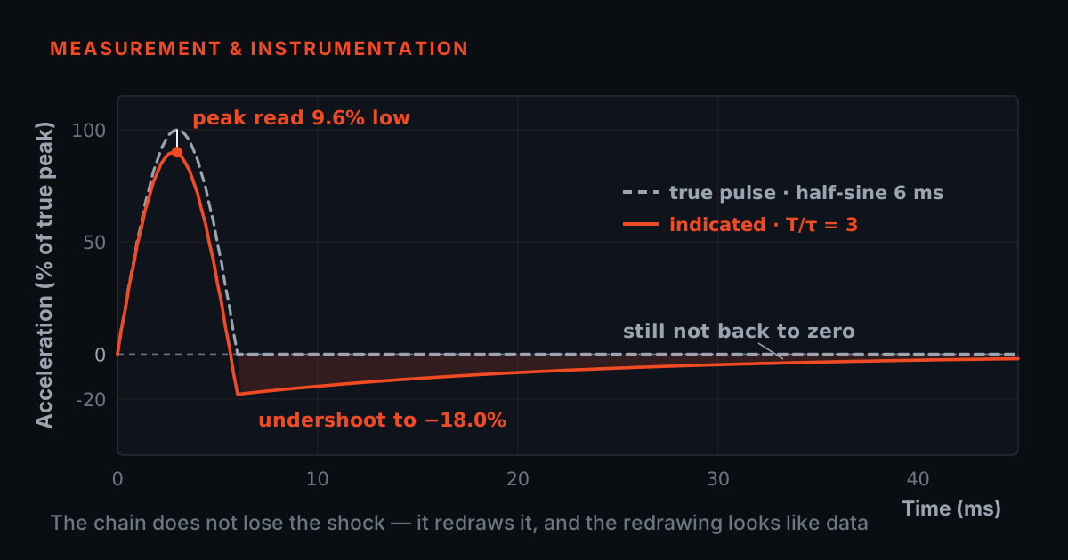
At the bottom, the low-frequency corner of the chain matters more than it does for steady vibration, because a transient contains content all the way down to DC. Too high a high-pass corner and the recorded pulse acquires an undershoot and a drifting baseline that were not in the event, which then propagates straight into the soft, residual-dominated end of the SRS — the end that is governed entirely by the velocity change, and therefore by the area under the pulse. Distort the area and you have distorted the answer. That family of errors, including the several distinct mechanisms behind an apparent zero shift after a hard shock, is enough of a subject on its own that TIERA treats it in a separate companion note on shock measurement and zero shift.
The practical implications are unglamorous. Capture with enough bandwidth and enough sample rate that the pulse shape, not just its peak, is resolved. Record the whole event including a clean pre-trigger baseline and enough post-pulse ring-down that the residual maximum has actually happened before your record ends — the simulator uses two full oscillator periods past the end of the pulse for exactly this reason. Then state the damping ratio, the convention (maximax, or positive and negative separately) and the frequency range of the bank alongside the curve. An SRS without those three annotations is a picture, not a measurement.
TIERA instruments that do this work.

Vertical and Lateral Shaker Stands
The fixturing under a shock or vibration test — the part that decides whether the pulse you specified is the pulse the specimen actually saw.
- Lateral stand
- Lateral / horizontal excitation stand for horizontal and oblique input
- Vertical stand
- Vertical shaker stand for aircraft structures, panels and fixtures
- Force input
- Wire-stinger and fixture arrangements for cleaner force input
- Intended for
- Designed for modal, FRF, ODS and structural dynamics testing
- Mobility
- Mobile stand formats for quicker laboratory repositioning

PhonoVibe Series — Sound & Vibration DAQ
Captures the transient the SRS is computed from — the sample rate and bandwidth decide whether the stiff end of your spectrum is real.
- ADC resolution
- 24-bit
- PhonoVibe Q / O / HD
- 128 kHz · 0.5 Hz – 60 kHz · ±5 V input
- PhonoVibe D
- 48 kHz · 2 Hz – 20 kHz · ±10 V input
- Sensor power
- 24 V, 4 mA constant current (IEPE/ICP/CCLD)
- Connectivity
- USB, plug-and-play
From the TIERA store
The kit for this job
What we would actually put in front of someone doing the measurement this post describes — not the whole catalogue.
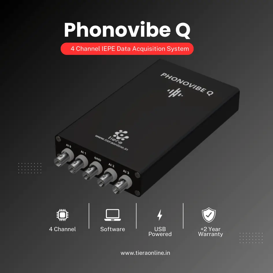 4 Channel IEPE Data Acquisition System – Phonovibe QFour Channels Standard plug & play USB Powered Take data from accelerometers, microphones, hammers, or any other IEPE Sensors T- VIB Software to acquire time waveforms, frequency spectra, overall vibration levels, FRF’s and octave measurements ** Windows 10 or above Operating System ** T-VIB Software base version comes with Time and Spectrum with Post processor TSAP 201. Check out TVIB Software regarding more module options.₹2,88,000View →
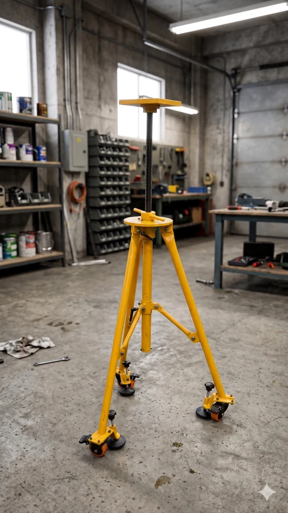 Vertical Shaker StandMechanical stand that positions an electrodynamic shaker for vertical excitation — safer handling, better alignment and repeatable force input for modal and structural dynamics testing.Request priceView →
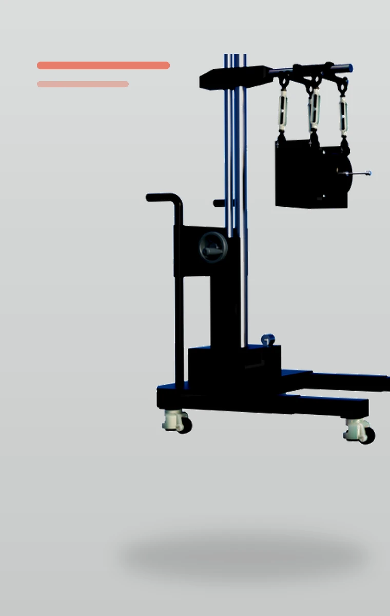 Horizontal / Lateral Shaker StandMechanical stand that adapts an electrodynamic shaker for horizontal and oblique excitation — safer handling, better alignment and repeatable force input for modal and structural dynamics testing.Request priceView →
Use cases
Where this shows up in the field
Shock work is a fixturing problem and a bandwidth problem before it is an analysis problem
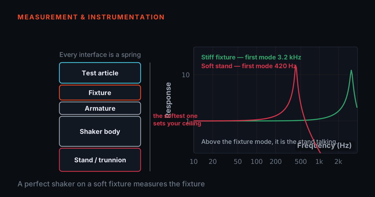
The two simulators on this page cost nothing to run and will not lie to you, because they compute rather than illustrate. What they cannot do is tell you whether the pulse your specimen actually experienced is the pulse you meant to apply. That is decided upstream, by how the excitation is introduced and by whether the recording chain was fast enough and wide enough to resolve the rise rather than just the peak.
TIERA supplies both ends of that chain. The shaker stand range positions electrodynamic shakers for vertical, horizontal and oblique input with wire-stinger and fixture arrangements for cleaner force input — the difference between exciting your specimen and exciting your fixture. PhonoVibe is the 24-bit USB DAQ that records what happened: the Q, O and HD models sample at 128 kHz across 0.5 Hz to 60 kHz, with IEPE sensor power and simultaneous sampling on every channel, so a short transient arrives with its shape intact and its channels time-aligned.
- Shaker stands — vertical, lateral and oblique excitation geometry for modal, FRF, ODS and structural dynamics testing
- PhonoVibe Q / O / HD — 128 kHz sampling, 0.5 Hz – 60 kHz, 24-bit, simultaneous sampling on every input
- IEPE / ICP / CCLD sensor power at 24 V, 4 mA with TEDS recognition
- Bundled TVIB TSAP 201 software for time waveform and narrowband analysis of the captured record
Where this sits on the TIERA learning ladder.
The theory behind this article is covered free, in full, by the TIERA 101 primers: Vibration 101 (Foundations), Accelerometer & DAQ Selection 101. They are self-paced, interactive, and end in an exam and a certificate.
The free 101 primers at 101.tieraonline.in cover the SDOF response and the measurement chain that everything on this page rests on — they are learning material, not an accredited ISO certification. The formal TCAT programme (see /services) adds structured Cat-level coursework and proctored examinations at exams.tieraonline.in for teams that need assessed, certificated competence.
TIERA 101 is a free introductory primer, not an accredited ISO certification, and its hours do not count towards the formal training ISO 18436 requires.