Run It Up Yourself: Drive a Machine Through Resonance on a Live Campbell Diagram
A hands-on companion to our resonance-or-forcing explainer. Drag the running speed, set one or two natural frequencies and a damping level, and watch forcing lines cross structure lines on a Campbell diagram while an honestly-computed response curve shows the shudder build and fall away.
You have already run this experiment
Put a washing machine into spin and listen. Somewhere on the way up it hits one particular speed and shudders hard enough to walk — then, a few hundred RPM later, it settles and runs smooth and fast. Nothing broke and nothing was fixed. The drum's once-per-revolution shaking force simply climbed through the one frequency at which the machine's own structure loves to vibrate, and carried on past it.
Our earlier explainer, Is It Resonance, or Is It the Force?, tells that story and gives the two field tests — the bump test and the coast-down — that settle a real diagnosis. This post is its hands-on companion. Instead of reading about a run-up, you get to drive one: a live diagram where you drag the speed, move the natural frequencies, turn the damping up and down, and feel the shudder zone arrive and pass under your own hand.
The map: a Campbell diagram
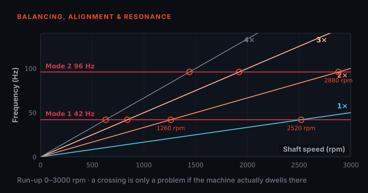
- Forcing lines fan up from the origin at their order; natural frequencies run flat, because mass and stiffness do not care what speed the rotor runs at.
- A crossing is not automatically a disaster. Crossings are the complete list of speeds where a disaster is available.
Engineers plot this situation on a Campbell diagram, and it is far simpler than its name suggests. The horizontal axis is running speed; the vertical axis is frequency. Every forcing mechanism tied to rotation draws a straight line fanning out from the origin: the 1× line for unbalance climbs at one cycle per revolution, the 2× line for misalignment climbs twice as fast, and a blade-pass line for a fan with eight blades climbs eight times as fast. Speed up the machine and every one of these lines rises with you.
The structure's natural frequencies draw the other family: flat horizontal lines, because mass and stiffness do not care what speed the rotor runs at. Every place a rising forcing line cuts a flat structure line is an interference — a speed at which that forcing mechanism lands exactly on that natural frequency. Crossings are not automatically disasters; they are the complete list of speeds where a disaster is available.
Drive it: the resonance explorer
The simulator below is that diagram brought to life. The top panel is the Campbell diagram: drag the speed slider and a cursor moves across it, with dots riding up the 1× and 2× lines (and an optional 8-blade blade-pass line). The dashed flat lines are natural frequencies you position yourself — one mode or two. The bottom panel is the part a paper Campbell diagram cannot show: the actual amplification at every speed, computed live from the same physics a vibration engineer would use.
Sweep the speed slowly and watch the two panels together. As the cursor approaches a crossing the response climbs; on the crossing it peaks; past it, it falls away — the washing-machine story in miniature. Then drag the damping slider up and sweep again: the same crossing is still there on the map, but the peak under it collapses and broadens. That is the whole art of resonance management on one screen — move the crossings, or damp the peaks.
The honest maths under the sliders
- At the crossing r = 1, the stiffness and inertia terms cancel exactly and only damping is left holding the response down: M(1) = 1 ÷ (2ζ).
- 1 ÷ (2ζ) is what ONE forcing line does at ITS own resonance. The response panel plots the whole machine — every order against every natural frequency — which is why the two numbers differ.
- Well above a crossing the inertia term dominates and the response falls below where it started. That is why the washing machine runs smoothest at full spin.
The response panel is not a cartoon. At every speed the simulator computes the standard single-degree-of-freedom magnification factor, M = 1 ÷ √[(1 − r²)² + (2ζr)²], where r is the ratio of forcing frequency to natural frequency and ζ is the damping ratio. Each forcing line (1×, 2×, blade-pass) is evaluated against each natural frequency, weighted, summed, and divided by the static response — so the readout is a true dynamic-over-static amplification, not a shape drawn to look right.
Read that number for what it is, because it is deliberately not the textbook figure printed beside the damping slider. 1 ÷ (2ζ) is what ONE forcing line does at ITS own resonance; the response panel plots what the whole machine is doing at that speed — every order against every natural frequency, over the static response of the same set. On the defaults (5% damping, modes at 24 and 42 Hz, 1× and 2× forcing) the 1× crossing with the first mode is worth ×10 on its own line and reads ×4.7 as a whole-machine average, which is where the status line starts calling it shuddering. Turn the second mode off and the same crossing reads ×7.5, because there is now half as much static compliance to divide by.
The formula explains what your hands feel on the sliders. Well below a crossing, r is small and M is close to 1: the structure follows the force stiffly and nothing dramatic happens. Right at the crossing, r = 1, the stiffness and inertia terms cancel exactly, and only the damping term is left holding the response down: M(1) = 1 ÷ (2ζ) exactly, so 5% damping means a tenfold magnification of whatever force is present. The curve's true maximum sits fractionally below the crossing, at r = √(1 − 2ζ²) — for any damping light enough to matter in the field the two are indistinguishable, which is why engineers treat r = 1 as 'the peak' as a matter of course. Well above the crossing the inertia term dominates and the response falls below where it started, which is exactly why the washing machine runs smoothest at full spin.
What damping actually buys you
- Damping does two things at once: doubling it halves the worst-case magnification, and it widens the peak — the band above 70.7% of maximum spans roughly 2ζ times the natural frequency.
- Light damping gives a needle a machine can sprint through on run-up; heavy damping gives a low mound that is gentle everywhere and quick to pass through nowhere.
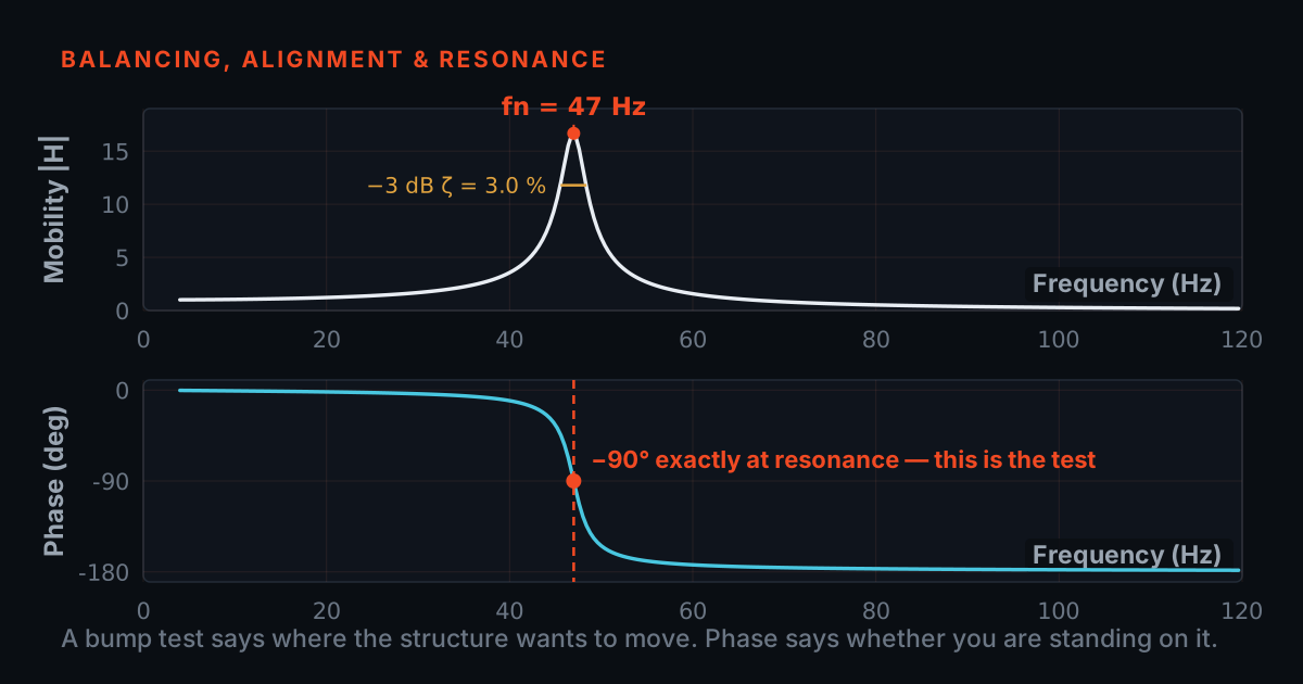
- Peak width is a measurement, not an appearance — it is how the damping ratio of a mode is estimated from a coast-down or an FRF.
Play with the damping slider and two things happen at once, and both matter in the field. The peak drops — 1 ÷ (2ζ) means doubling the damping halves the worst-case magnification. And the peak widens: the band of speeds over which the response exceeds 70.7% of its maximum spans roughly 2ζ times the natural frequency. Light damping gives a tall, needle-thin spike that a machine can sprint through during run-up almost unharmed; heavy damping gives a low, broad mound that is gentle everywhere but quick to pass through nowhere.
That width is also a measurement you can take. On a real coast-down or FRF, the sharpness of a resonance peak is how engineers estimate the damping ratio of a mode — the half-power bandwidth method. A structure whose peak is razor-sharp on the analyser is telling you it has almost no damping to protect it, and that running anywhere near that crossing is a standing invitation to the kind of repeat-balancing misery the first post described.
From simulator to machine — and where to learn more
A representative case, not a specific customer: a plant upgrades a fan drive to a variable-frequency drive so operators can trim flow with speed. On the old fixed-speed motor the fan ran quietly for years; with the VFD, certain setpoints shake the ductwork alarmingly while others are fine. In simulator terms, the old motor parked the cursor at one safe spot between crossings — the VFD handed operators the speed slider, and some setpoints land squarely on interferences that were always on the map. The fix is the same as in the sim: identify the crossings with a coast-down or bump test, then either block out the offending speed bands in the drive, shift the natural frequency by stiffening, or add damping so the remaining peaks are survivable.
If this post made the picture click, the theory behind it is covered in TIERA's free primers at 101.tieraonline.in — start with Modal & Resonance 101, which walks through natural frequencies, mode shapes and damping from zero. The primers are free introductions, not accredited ISO certifications. For formal, career-grade training, TIERA's TCAT programme (see /services) runs structured courses with proctored certification exams at exams.tieraonline.in.
TIERA instruments that do this work.

PhonoVibe Series — Sound & Vibration DAQ
Captures the real version of the sweep — coast-downs, run-ups and bump tests that carry the forcing line through your structure's natural frequencies, two channels and up.
- ADC resolution
- 24-bit, simultaneous sampling
- Channels
- 2, 4, 8 or 16 (BNC)
- Bandwidth (Q/O/HD)
- 0.5 Hz – 60 kHz at 128 kHz
- Sensor power
- 24 V, 4 mA (IEPE/ICP/CCLD)
- Calibration
- Factory certificate, 1-year validity
TWGM 206 — Waveform Generator
Puts the excitation under your control instead of riding on residual unbalance: clean sine sweeps and bursts into a shaker for measured FRF response curves like the sim's bottom panel.
- Sine sweep
- Linear and logarithmic, plus sweep burst for FRF
- Noise
- Pink, white and random, with noise burst
- Band limiting
- Bandpass filter on noise output
- Drives
- T-Xcite series shakers and amplifiers
- Integration
- Runs inside TVIB, output via PhonoVibe DAC

Vertical and Lateral Shaker Stands
Holds the shaker in a repeatable geometry — vertical, horizontal or oblique — so the FRF you measure reflects the structure, not the day's improvised rig.
- Orientations
- Vertical, horizontal and oblique excitation
- Force input
- Wire-stinger and fixture arrangements
- Formats
- Mobile stand formats for quicker repositioning
- Intended for
- Modal, FRF, ODS and structural dynamics testing
From the TIERA store
The kit for this job
What we would actually put in front of someone doing the measurement this post describes — not the whole catalogue.
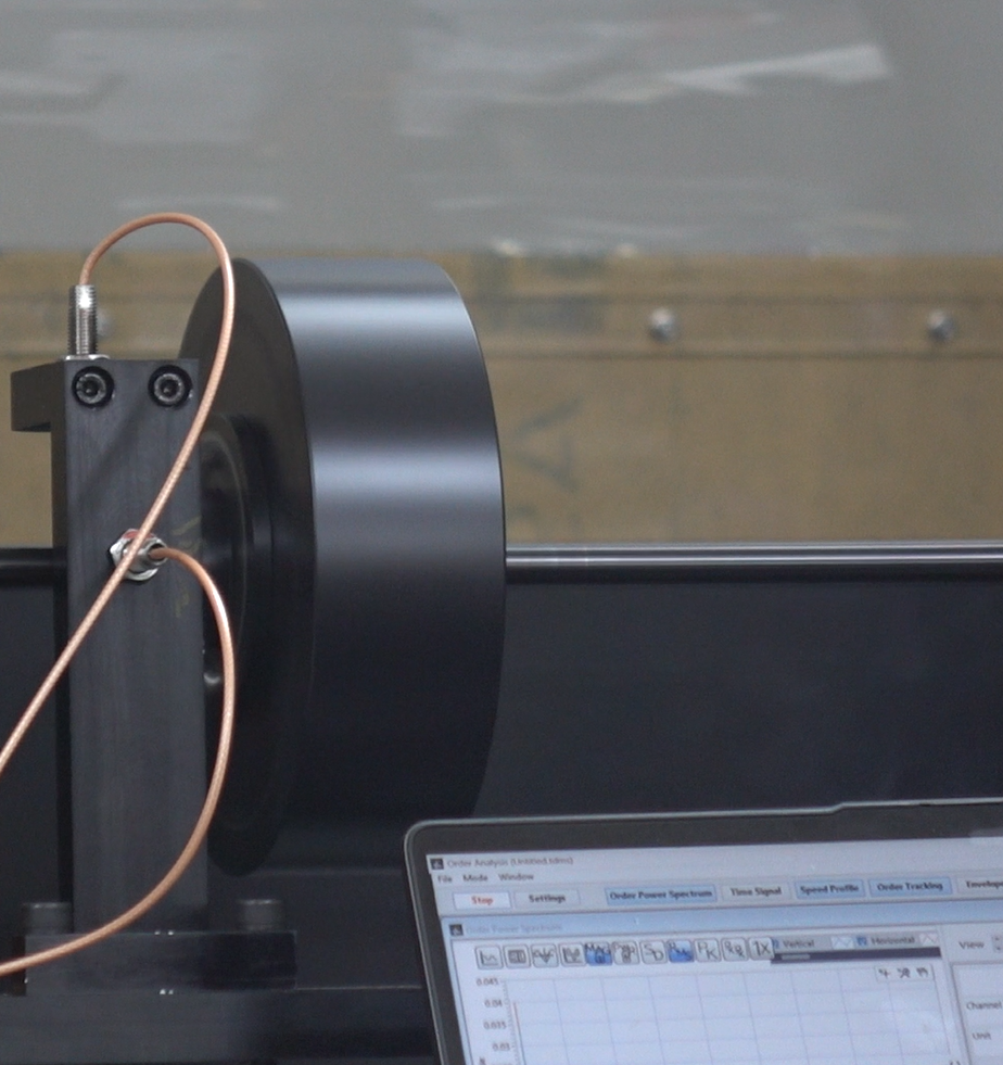 Resonance Simulation KitResonance Faults Addon Kit for the TMFSS Macro simulates resonance-related faults in industrial machines₹1,87,500View →
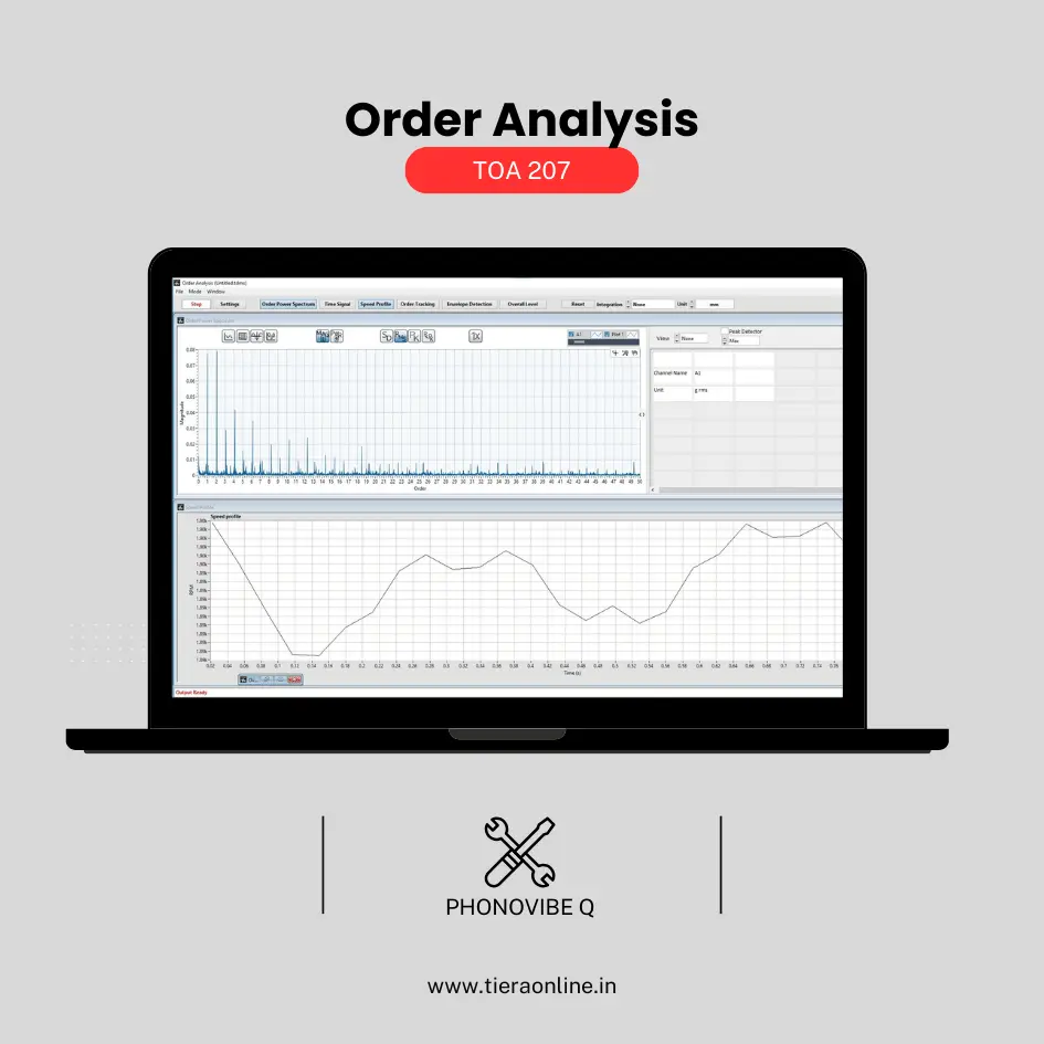 TOA 207 – Order Analysis(Phonovibe Q)Use Cases Machine Condition Monitoring Run up Coast Down Test₹57,600View →
 4 Channel IEPE Data Acquisition System – Phonovibe QFour Channels Standard plug & play USB Powered Take data from accelerometers, microphones, hammers, or any other IEPE Sensors T- VIB Software to acquire time waveforms, frequency spectra, overall vibration levels, FRF’s and octave measurements ** Windows 10 or above Operating System ** T-VIB Software base version comes with Time and Spectrum with Post processor TSAP 201. Check out TVIB Software regarding more module options.₹2,88,000View →
Use cases
Where this shows up in the field
The simulator shows the idea — your machine has its own Campbell diagram, and we build the kit to measure it.
Everything the explorer fakes with sliders is measurable on real machines. A coast-down or run-up captured on a PhonoVibe DAQ — two channels is enough to start — sweeps the forcing line through your structure's natural frequencies for free, and a bump test on the stopped machine confirms them. TVIB's TSAP201 spectrum analyser reads the peaks, and its FRF modules (TFRT, TIST 205) measure the response curve you saw in the bottom panel, including the damping that sets peak height and width.
For lab and development work, where you want the excitation under your control rather than riding on residual unbalance, a shaker on a TIERA vertical or lateral stand driven by the TWGM 206 waveform generator gives clean sine sweeps, bursts and shaped noise through the same PhonoVibe-and-TVIB chain — the full measured version of this page.
- PhonoVibe 24-bit USB DAQ (2 to 16 channels) for coast-down, run-up and bump-test capture in the field
- TVIB software — TSAP201 spectrum analysis bundled free; FRF and modal modules when you need the full response curve
- TWGM 206 waveform generator for controlled sine sweeps, bursts and band-limited noise into a shaker
- Vertical and lateral shaker stands for repeatable excitation geometry in the lab
Where this sits on the TIERA learning ladder.
The theory behind this article is covered free, in full, by the TIERA 101 primers: Modal & Resonance 101. They are self-paced, interactive, and end in an exam and a certificate.
TCAT adds instructor-led training on Campbell diagrams, modal testing and resonance correction, with proctored certification exams at exams.tieraonline.in — the free 101 primers introduce the ideas but are not accredited certifications.
TIERA 101 is a free introductory primer, not an accredited ISO certification, and its hours do not count towards the formal training ISO 18436 requires.