Why a Shock Reading Lies — and How to Tell That It Lied
A transient gets no second chance: you record it once, and every distortion the chain adds arrives looking exactly like data. Two live simulators — drive the high-pass time constant until the error crosses 5% and 2% and read the ratio you need, then take the sensor over range and watch the baseline walk off zero while the integrated velocity marches away.
A transient gets exactly one chance
- A record mangled by its own instrumentation does not look mangled. It looks like a slightly different shock, and there is no second event to check it against.
- Two failure families account for nearly all of it: a linear high-pass error you can calculate in advance, and zero shift — five unrelated faults wearing one symptom.
Steady vibration is forgiving. If a spectrum looks wrong you average again, change the window, move the sensor and re-measure; the machine keeps producing the signal while you argue with it. A shock does not wait. A drop test, a rail impact, a gunfire event, a package fall, a punch press strike — it happens once, in a few milliseconds, and whatever the measurement chain wrote down is now the only evidence that the event occurred at all.
That asymmetry is the whole problem. Every distortion the chain introduces on a transient arrives in the file looking exactly like acceleration. There is no second record to compare it against, no averaging to push it down, and — this is the part that catches people — nothing in the data announces itself as an artefact. A shock record that has been mangled by its own instrumentation does not look mangled. It looks like a slightly different shock.
Two families of error account for most of it. The first is linear and completely predictable: the chain's own low-frequency roll-off, which cannot pass a signal that has a net area, so it invents an undershoot and an apparent baseline offset to make the area cancel. The second is a group of five separate faults that share one symptom — the trace does not return to zero after the event — and are collectively called zero shift. Four of them are electrical and one is mechanical, which matters because the fix is different in each case.
This post derives the first from a first-order model you can drive yourself, names the five causes of the second, and finishes with the checks that separate a real shock from a chain that lied about one.
Why a high-pass cannot tell the truth about a pulse
- A first-order high-pass has zero net area at its output, so it must draw an undershoot lobe whose area equals the pulse's exactly.
- The time constant does not decide whether that lobe exists, only what shape it takes — and a short one steals height off the peak on the way through.
- Everything that follows depends on one ratio and nothing else: the chain time constant T over the pulse duration τ.
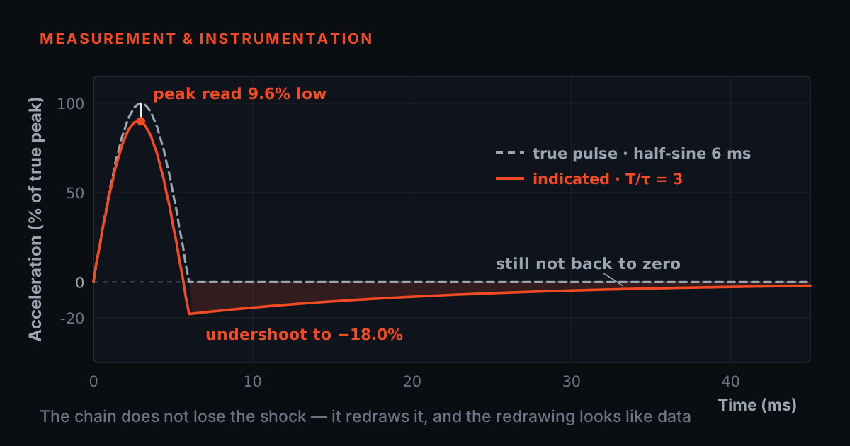
Almost every measurement chain is AC-coupled somewhere. The charge amplifier has a finite discharge time constant; the IEPE conditioner has a DC-blocking capacitor; the recorder has an input coupling capacitor of its own. Each of those is a first-order high-pass, and a first-order high-pass has one property that is fatal to transients: its output has zero net area. Whatever goes up must come down, and the areas must cancel exactly.
That is not a design flaw, it is arithmetic. The transfer function is H(s) = sT/(1 + sT), so H(0) = 0, so the DC component of the output is zero, so the integral of the output over all time is zero. A shock pulse, however, has a very large net area — that area is the velocity change the event imparted. A 100 g half-sine lasting 6 ms carries (2/π)(100)(9.80665)(0.006) = 3.75 m/s of velocity change. The high-pass has to get rid of all of it.
It does so by drawing an undershoot lobe below zero whose area equals the pulse's area exactly, no matter what the time constant is. What the time constant controls is not whether the lobe exists but what shape it takes. A long time constant spreads that 3.75 m/s over hundreds of milliseconds as a barely-visible sag. A short one crams the same area into a deep, obvious dip immediately after the event — and steals height off the peak on the way through, because the droop has already started before the pulse has finished.
So the requirement is not "AC coupling is bad". It is a ratio. Call the pulse duration τ and the chain's high-pass time constant T. Everything below depends on T/τ and on nothing else.
Try it: how much time constant does a pulse actually need?
The simulator below is the model and nothing but the model: one first-order high-pass applied to one of three canonical pulse shapes. Pick a shape, set the pulse duration and the chain time constant, and it draws the true pulse against the indicated one, shades the undershoot lobe, and prints the peak error, the worst error anywhere inside the pulse, the depth of the dip, and the area of the lobe expressed as a velocity change in m/s.
The lower plot is the one to spend time on. It sweeps T/τ from 1 to 1000 and plots the worst in-pulse error, with the 5% and 2% acceptance lines drawn across it and the crossing ratios labelled. Drag the time constant slider and watch the orange dot travel along that curve and cross the lines. The crossing ratios are not typed into this page: they are solved by bisection on the same model that draws the waveform, every time you change pulse shape.
Drive it and three results fall out. First, the ranking of pulse shapes is a ranking of areas. The worst error scales as roughly 100k/(T/τ), where k is the pulse's area as a fraction of peak-times-duration: 1 for a square, 2/π ≈ 0.637 for a half-sine, 0.5 for a terminal-peak sawtooth. So to hold the worst in-pulse error under 5% you need T/τ ≈ 19.5 for a square, ≈ 12.2 for a half-sine and ≈ 9.7 for a sawtooth; for 2% those become ≈ 49.5, ≈ 31.3 and ≈ 24.7. Read them off the lower plot yourself — they will match.
Second, the square pulse is the worst case, which makes it the useful one to design against. If you size the chain's low-frequency response on the assumption of a square pulse of your expected duration, no half-sine or sawtooth of the same duration can do worse. That sizing argument is the core claim of Endevco TP214, "The Accurate Measurement of Shock Phenomena"; the ratios above are our own, computed here, not taken from it.
Third, peak error and waveform error are not the same measurement. Switch to the square pulse and watch the peak error sit stubbornly at 0.00% while the worst error climbs past 10%. That is not a bug: a square pulse's peak happens at t = 0, before the droop has had time to accumulate, so a peak-only readout reports a perfect number on a badly distorted record. If your acceptance criterion is peak g, a square-ish pulse will pass it while the waveform underneath is wrong — and the velocity you derive from that waveform will be wrong with it. For a half-sine the peak error crosses 5% at T/τ ≈ 6.0 and 2% at ≈ 15.6, roughly half the ratio the full waveform needs.
The model is one first-order high-pass, y[n] = α(y[n−1] + x[n] − x[n−1]) with α = e−Δt/T. Every figure above is computed from it live, including the 5 % and 2 % crossing ratios, which are solved by bisection on this same model rather than read from a table. The corner-frequency chips assume the stated corner is a single first-order high-pass, so that T = 1/(2πfc); a steeper or multi-stage roll-off behaves worse than this, not better.
Time constants add the way resistors in parallel do
A real chain has more than one high-pass in it. The sensor or charge amplifier has a discharge time constant; the conditioner has a coupling capacitor; the recorder input has another. It is tempting to assume the longest one governs. It is the opposite: the shortest dominates, and the rest still make it worse.
Because the error is set by how much of the pulse's area leaks away per unit time, and each stage leaks independently, the reciprocals add: 1/Teff ≈ 1/T₁ + 1/T₂ + … A 20τ stage followed by a 30τ stage behaves like a single 12τ stage. You can check that in the simulator: set T/τ = 12 for a half-sine and the worst error is about 5.1%, which is what the two-stage cascade actually produces. Three innocuous-looking stages of 60τ each are one bad stage of 20τ.
This is also why a stated "low-frequency corner" needs reading carefully. If a specification says the response is flat down to a corner fc and that corner is a single first-order high-pass, then T = 1/(2πfc) and the chips in the simulator apply: 0.5 Hz is 318 ms, 2 Hz is 79.6 ms, 20 Hz is 7.96 ms. If instead the corner is a steeper multi-pole roll-off, the pulse fares worse than this model predicts, not better — extra poles mean extra phase distortion on top of the area loss.
The practical consequence is simple. Total the reciprocals for your actual chain, divide into your shortest expected pulse, and compare with the crossing ratio the simulator gives for your pulse shape. For a 1 ms pulse — not unusual in impact and pyroshock work — 2% on a half-sine needs T ≥ 31 ms, which almost anything satisfies. For a 50 ms pulse, the same 2% needs T ≥ 1.57 s, and now the 318 ms of a 0.5 Hz corner is nowhere near enough. Long, gentle pulses are the ones AC coupling ruins, not short sharp ones.
Which points at the real fix where it is available. If the instrument can be DC-coupled, the whole first-order problem disappears from everything downstream of the sensor, and only the sensor's own time constant remains. Every PhonoVibe model supports static (DC) measurements, so on that hardware this is a configuration decision rather than a purchase.
Zero shift: five faults wearing one symptom
- The symptom is identical in all five cases — the trace does not come home to zero — but the causes are unrelated, and only the first is calculable, bounded and correctable in advance.
- Four happen downstream of the crystal and can be re-configured, re-cabled or re-filtered. The fifth happens inside the ceramic, so the sensor genuinely produced that offset and nothing can undo it.
The symptom is always the same — after the event, the trace sits at some level that is not zero, and creeps back over a time far longer than the shock. The causes are unrelated to each other, and four of them are electrical while one is not.
1 · Insufficient time constant (electrical, and predictable). The one derived above. This is the benign case, and the only one you can calculate in advance, bound, and even correct for after the fact. It is also the only one whose offset is guaranteed to decay with a known constant. Everything below is worse because it is none of those things.
2 · Amplifier clipping and nonlinearity (electrical). Drive an amplifier past its linear range and two things happen. The obvious one is that the peak is truncated, so the recorded peak is simply wrong. The dangerous one is that the stage's operating point is disturbed and recovers on a time constant of its own — typically far longer than the event — so after the shock the output sits at an offset that has nothing to do with acceleration. Because shock spectra contain very high-frequency content (the accelerometer's own mounted resonance rings hard on any step), the stage can be driven into saturation by energy you never intended to measure and are not even looking at in the final record.
3 · Triboelectric cable noise (electrical, generated mechanically). When a coaxial cable is flexed, struck, or whipped, friction between the dielectric and the shield separates charge, and that charge appears at the amplifier input as a signal. In steady vibration it is a nuisance in the low-frequency end of the spectrum. In shock it is far worse, because the cable gets whipped by the very event you are measuring, at exactly the moment you are measuring it, producing a low-frequency excursion that is indistinguishable from acceleration. The fixes are mechanical: low-noise treated cable, and clamping or taping the cable to the structure within a few centimetres of the sensor so the run near the connector cannot move.
4 · Filter ringing (electrical). A sharp anti-alias or band-limiting filter with non-linear phase does not simply remove high frequencies from a step — it rings. The tail of that ringing rides on the record after the pulse and can be mistaken for structural response or for an offset. It also produces the one artefact that is genuinely diagnostic: a precursor, a wiggle appearing before the pulse arrives. No mechanical input can do that. If you see energy ahead of the event, you are looking at your filter.
5 · Ferroelectric domain relaxation in the ceramic (mechanical — and this one is not fixable downstream). A poled piezoceramic holds its sensitivity because its ferroelectric domains are aligned. A sufficiently large, sustained mechanical load can partially re-orient them. The crystal's own charge state then shifts, and what comes out of the sensor already contains an offset before any cable, amplifier or filter has touched it. No conditioner setting, no filter, and no post-processing can undo it, because the sensor genuinely produced that signal. Endevco TP213, "Shock Motions and Their Measurement" is where this mechanical cause is set out alongside the four electrical ones above.
The design consequence is a sensor choice, not a settings change. Compression-design piezoelectric accelerometers show sensitivity that rises with acceleration level and are the most prone to this; shear designs hold linearity far better at high level; piezoresistive accelerometers, whose output is a resistance change rather than a stored charge, do not exhibit a comparable zero shift at all — which is why they are the recommended choice when the shock record is going to be integrated to velocity or displacement. That comparison is the substance of Endevco TP250, "Accelerometer Characteristics Used in Transient Motion and Nuclear Applications".
Try it: over range, and the baseline that walks away
The second panel takes the sensor over range. A 2 ms half-sine is measured against a 500 g full-scale over a 40 ms record — all illustrative figures, chosen so the arithmetic is easy to check by hand — and there are three controls: the true peak of the event, the size of the zero shift the over-range leaves behind, and the chain time constant.
Start below full scale, at the default 300 g. The record tracks the pulse, and the velocity underneath does what a real finite event must do: rises during the pulse and then settles onto a shelf. A shock of finite duration imparts a finite velocity change and then stops; that shelf is the physical signature of a genuine transient. It is not perfectly flat — it sags by about 4% across the 40 ms window, which is exactly the linear high-pass effect from the first panel, bounded and predictable. Drag the time constant down and watch that sag grow; that part you can calculate.
Now push the peak to 600 g with the zero shift still at zero. The top of the pulse flattens off at 500 g, the peak reads 16.7% low, and the shelf lands at 6.74 m/s against a true 7.49 m/s. That is clipping alone, and it is at least an honest error: a flat top is visible to anyone who looks at the waveform.
Then add zero shift. Two per cent of full scale is 10 g — a hair's breadth above the zero line on a plot scaled for 500 g, and easy to dismiss as baseline wander. But 10 g held for 40 ms is 10 × 9.80665 × 0.040 = 3.92 m/s of velocity that never happened. The velocity trace stops settling and starts marching: 10.39 m/s against a true 7.49 m/s, a 39% overestimate from an offset you cannot see. Push the shift to the top of its slider, 5% of full scale, and the offset alone contributes 9.81 m/s — more velocity than the shock itself delivered.
One more thing worth doing, because it is the trap: set the peak to 1500 g and leave the shift at 2%. The peak now reads 66.7% low from clipping while the zero shift pushes the velocity up, and the two errors partly cancel — the record comes out at 12.07 m/s against a true 18.73 m/s, a plausible-looking 36% low. Two large errors in opposite directions can produce a number that looks merely disappointing rather than wrong. Never read the size of the error off how reasonable the answer looks.
That is the whole diagnostic, and it is why this panel plots the integral rather than just the acceleration. You cannot see a small zero shift on an acceleration trace scaled for a large shock. You cannot miss it on the integral. Extend the record long enough and the offset does decay with the chain time constant — try dragging that slider — but it decays over hundreds of milliseconds, which is to say long after any window in which the velocity number was supposed to mean something.
The 500 g full-scale range, the 2 ms half-sine and the 40 ms record window here are illustrative, not a TIERA specification. Clipping is modelled as hard truncation at full scale. The zero shift is a control, not a prediction: the size of a real zero shift is not a known function of how far you exceeded range, which is exactly what makes it dangerous — so this panel lets you set it and watch what it does to the data.
Seven checks that catch a lying record
- Integrate the record. A genuine finite-duration shock gives a velocity that rises and settles onto a shelf; a contaminated one gives a velocity that ramps and never settles inside the window.
- Energy before the pulse is the one unambiguous artefact — causality rules out every mechanical explanation, so it can only be your filter.
- Check the peak against the sensor's rated range, and remember the amplifier saw the mounted-resonance ringing that your filtered record no longer shows.
None of these needs special equipment. Most of them are things you can do to a file you have already recorded.
1 · Integrate it. The single most useful test there is. A genuine finite-duration shock produces a velocity that rises and then settles onto a shelf. A record contaminated by zero shift produces a velocity that ramps and does not settle inside the window. If your analysis software will not integrate a transient, do it in a spreadsheet — it is a cumulative sum times the sample interval.
2 · Compare the undershoot area with the pulse area. For a linear high-pass they must be equal, because the output's net area is zero. If the dip after your pulse carries visibly more or less area than the pulse itself, the offset is not coming from AC coupling — it is coming from one of causes 2 to 5, and you have just eliminated the benign explanation.
3 · Check the peak against the sensor's rated range, not against what looks reasonable. Over-range is the precondition for both clipping and domain relaxation. And remember the peak you must check is not the peak in your filtered record: the sensor sees its own mounted resonance ringing on the impact, which can be several times the peak of the pulse itself and is removed later by the anti-alias filter. The amplifier saw all of it.
4 · Repeat the event at a lower level. A linear chain scales: halve the input, everything halves. Clipping, saturation recovery and domain relaxation are threshold phenomena — they appear abruptly and disappear abruptly. If the shape of your record changes when the level changes, the chain is not linear over the range you are using it.
5 · Record with no shock at all, and rattle the cable. Thirty seconds of data while someone flexes and taps the cable run will tell you immediately whether triboelectric noise is a factor for that installation. Then clamp the cable near the sensor and do it again.
6 · Look before the pulse. Any energy ahead of the event is your filter's precursor ringing, not the machine. This is the one artefact that is unambiguous, because causality rules out every mechanical explanation.
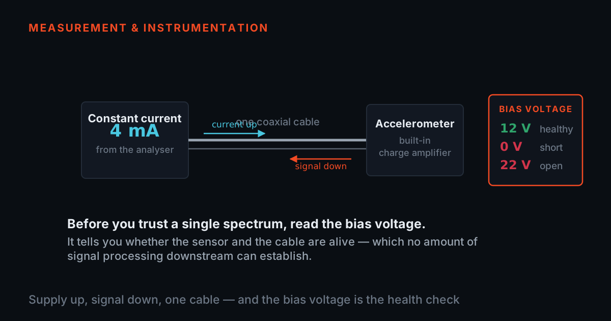
7 · Prove the chain's gain electrically, without a shock. An electrically insulated piezoelectric transducer allows a known voltage to be inserted in series with its ground return, simulating the charge the crystal would have generated and exercising every stage downstream of it. It verifies system gain end to end and finds opens and shorts without mechanical excitation — useful precisely when the event is expensive or single-use. The technique, and the conditions on the insertion resistor and the transducer's own capacitance, are set out in Endevco TP216, "Piezoelectric Transducer Calibration Simulation Method Using Series Voltage Insertion".
One more, for completeness: the sensor must be stiff enough to be treated as a rigid mass over the band the pulse occupies. The conventional requirement is that the accelerometer's own natural frequency sits at least about four times above the highest frequency component being measured — stated as such in Endevco TP213, "Shock Motions and Their Measurement". Below that, the sensor's own dynamics are part of what you recorded.
Setting a chain up so it does not lie in the first place
Work out the shortest pulse you expect and the shape closest to it, then use the simulator to get the T/τ your accuracy target needs. Total 1/T across every AC-coupled stage in the chain — sensor, conditioner, recorder — and check the total against that requirement, not each stage individually. If a DC-coupled path is available and your sensor supports it, take it; it removes every stage's contribution except the sensor's own.
Choose range with real headroom, and choose it against the ringing rather than the pulse. A sensor rated close to the expected peak will be driven past full scale by the mounted-resonance response to the impact even when the pulse itself is comfortably inside range. Where the record will be integrated to velocity or displacement, prefer a shear design over a compression design, and consider piezoresistive where the level is high enough that any zero shift at all would be fatal to the answer.
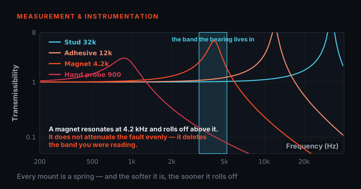
Mount stiffly and clamp the cable. A soft mount lowers the mounted resonance into the band the pulse occupies, and an unrestrained cable is a signal source in its own right during exactly the milliseconds that matter. Both are free.
Then record longer than you think you need. A window that ends shortly after the pulse cannot show you whether the baseline came home, which means it cannot distinguish a good record from a zero-shifted one. Ten to twenty times the pulse duration costs nothing and turns check 1 from impossible into trivial.
And keep the raw record. Every check above except the electrical insertion test is done on data you already have — but only if what you kept is the record and not a peak value extracted from it. A single number cannot be interrogated. A waveform can.
TIERA instruments that do this work.
TSP Series IEPE Signal Conditioners
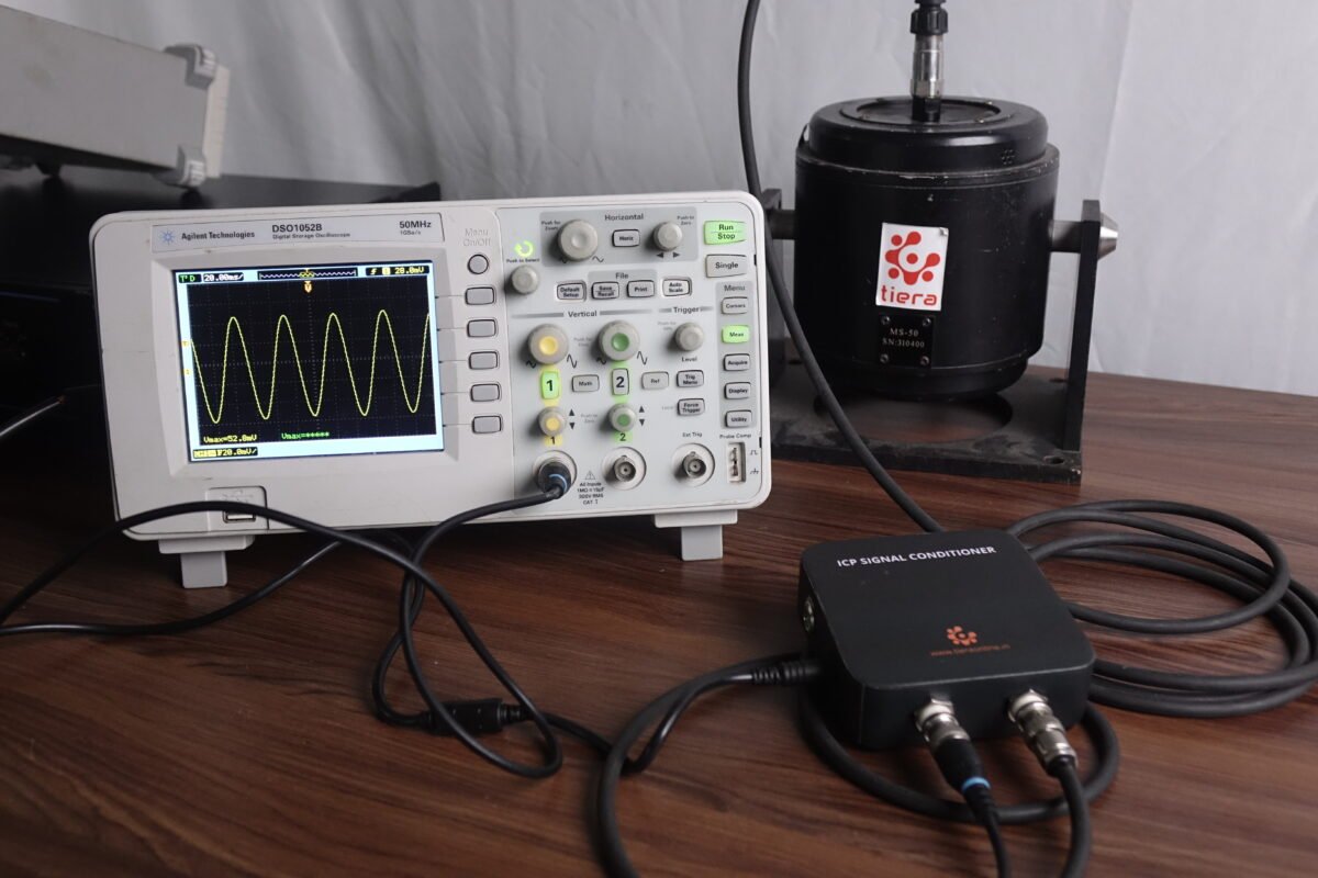
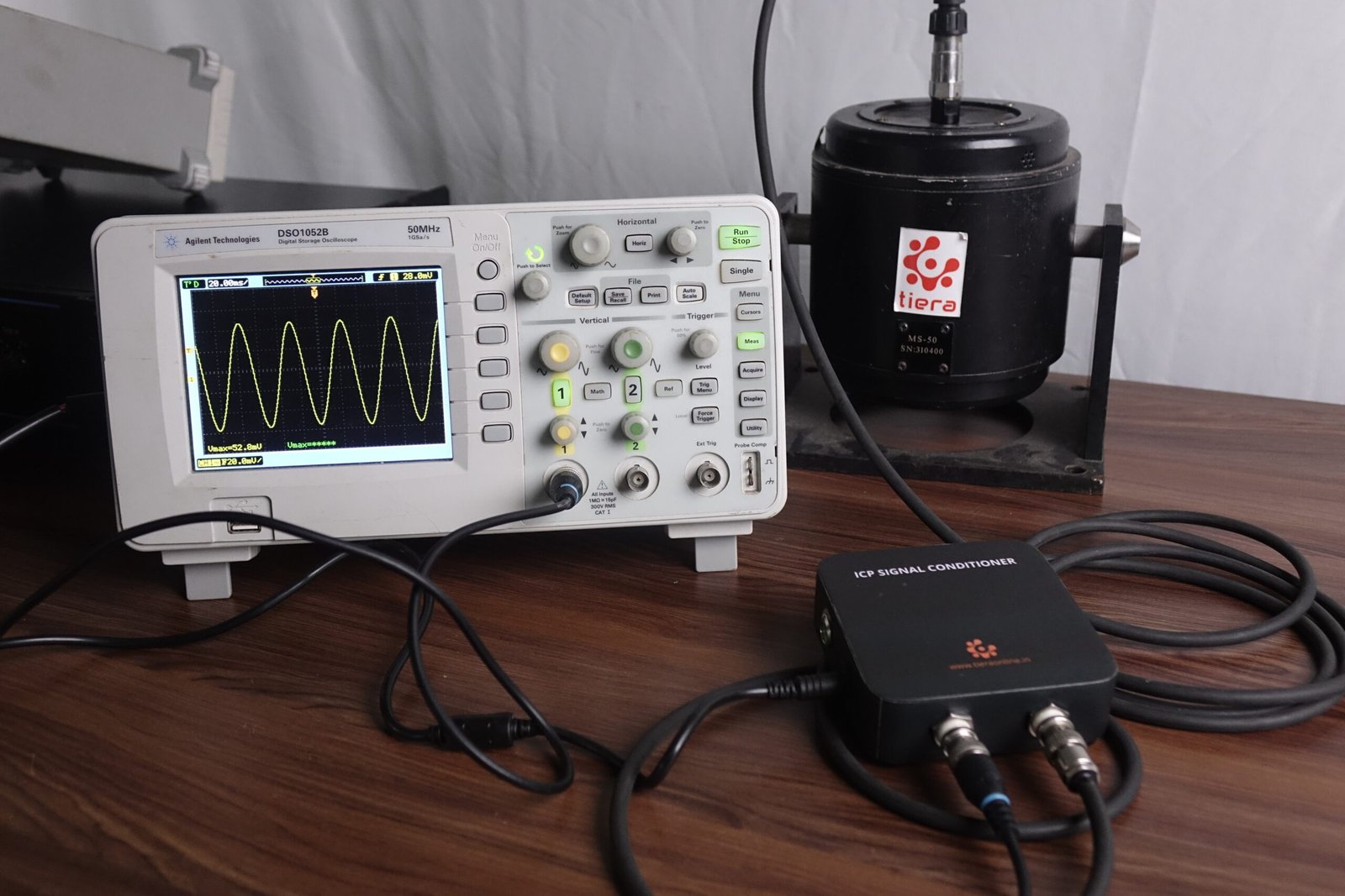
The stage where a shock chain's low-frequency corner is usually decided. The stated response starts at 0.5 Hz; treated as a single first-order high-pass that is a time constant of about 318 ms, which the simulator above turns into a T/τ for your pulse. Unity gain means the conditioner adds no gain stage to be driven out of range.
- Input type
- ICP® / IEPE
- Excitation
- 24 VDC, 4 mA constant
- Frequency response
- 0.5 Hz – 50,000 Hz
- Gain
- 1 (unity)
- Connectors
- BNC / BNC

PhonoVibe Series — Sound & Vibration DAQ
Static (DC) measurement is supported across the series, which is the one setting that removes the recorder's own high-pass from the argument entirely. Simultaneous sampling matters on a transient, where a channel-to-channel time skew is a phase error you cannot average away.
- ADC resolution
- 24-bit
- Static measurements
- Static (DC) measurements supported
- Sampling
- Simultaneous sampling on every input
- Sensor power
- 24 V, 4 mA constant current (IEPE/ICP/CCLD)
- Calibration
- Factory calibration certificate, 1-year validity
From the TIERA store
The kit for this job
What we would actually put in front of someone doing the measurement this post describes — not the whole catalogue.
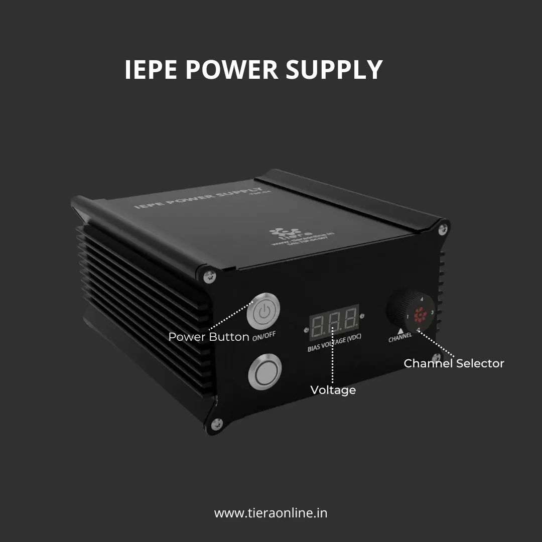
 TSP 02- Single Channel IEPE Power SourceLow Cost Customizable Connect ICP/IEPE Sensors to the oscilloscope or Voltage Input DAQ₹27,600View →
 Four Channel IEPE Power Source-TSP 04Low Cost Customizable Connect ICP/IEPE Sensors to the oscilloscope or Voltage Input DAQ₹54,000View →
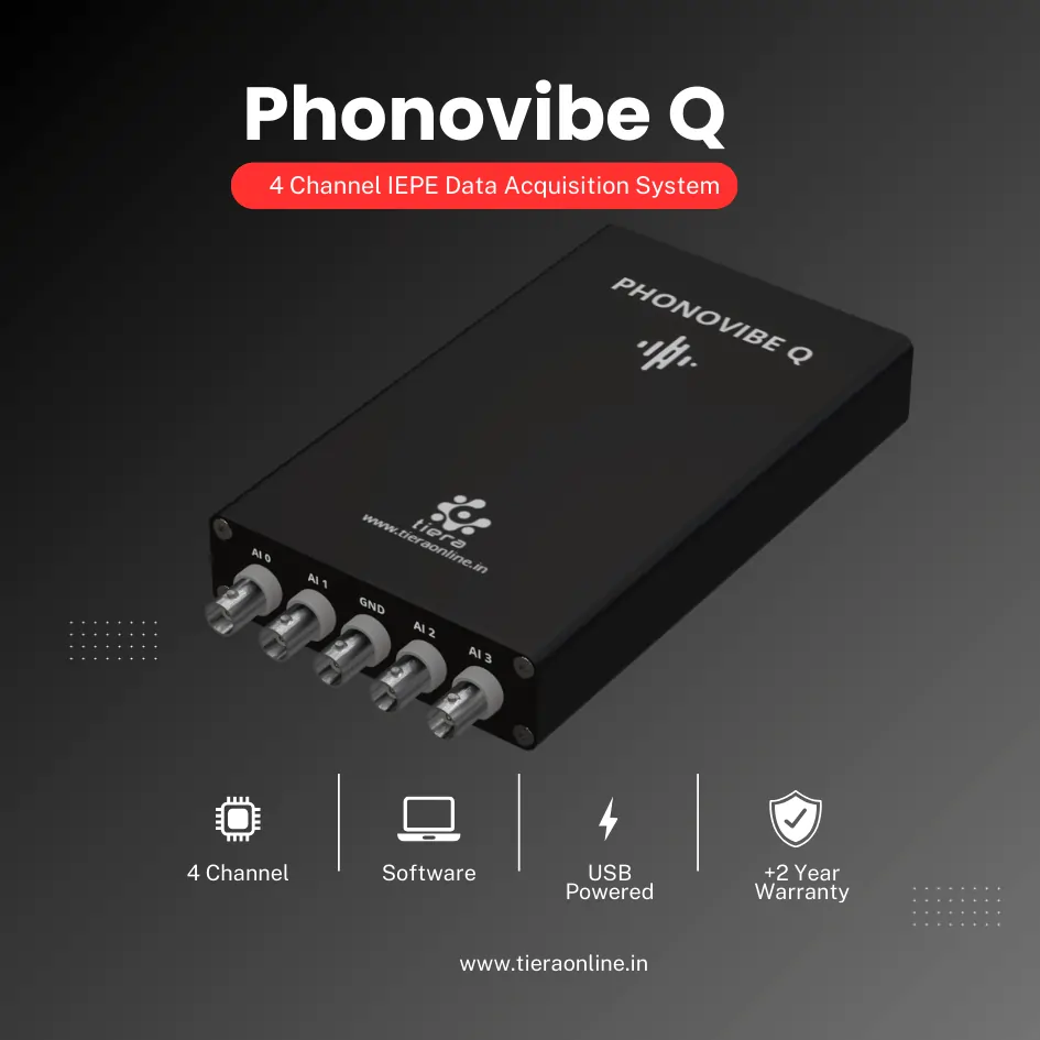 4 Channel IEPE Data Acquisition System – Phonovibe QFour Channels Standard plug & play USB Powered Take data from accelerometers, microphones, hammers, or any other IEPE Sensors T- VIB Software to acquire time waveforms, frequency spectra, overall vibration levels, FRF’s and octave measurements ** Windows 10 or above Operating System ** T-VIB Software base version comes with Time and Spectrum with Post processor TSAP 201. Check out TVIB Software regarding more module options.₹2,88,000View →
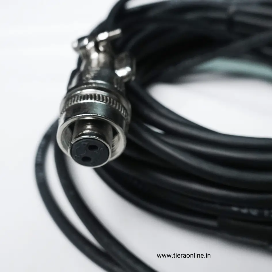 Accelerometer Sensor CableCA-102-5-D-B : Tinned Copper Braid 2 Core Twisted Shielded Cable – One side 2 Pin Circular MIL Connector other side BNC Connector₹1,500View →
Use cases
Where this shows up in the field
A shock you cannot repeat deserves a chain you have already checked.
The failure this article describes is silent by construction: the record looks like data, the peak looks plausible, and the only thing wrong with it is that the instrument wrote part of it. Sizing the low-frequency corner against the pulse, keeping range headroom against the ringing rather than the pulse, and recording long enough to see the baseline come home costs nothing at all — but it has to be decided before the event, not after.
TIERA supplies the conditioning and acquisition end of that chain and will talk through the pulse you actually expect before recommending anything. If your existing DAQ can be DC-coupled and your cables are already clamped, we will say so.
- TSP 02 and TSP 04 IEPE power sources — unity gain, 0.5 Hz – 50 kHz stated response
- PhonoVibe 2/4/8/16-channel 24-bit DAQ with static (DC) measurement and simultaneous sampling
- Cables and mounts specified for the run and the mounting stiffness the pulse needs
Where this sits on the TIERA learning ladder.
The theory behind this article is covered free, in full, by the TIERA 101 primers: Accelerometer & DAQ Selection 101, Measurement Setup 101. They are self-paced, interactive, and end in an exam and a certificate.
The primers cover the sensor and the chain that carries its signal. Reading a transient record critically — deciding whether an offset is the chain, the cable or the crystal, and what that means for a velocity derived from it — is Cat II and above.
TIERA 101 is a free introductory primer, not an accredited ISO certification, and its hours do not count towards the formal training ISO 18436 requires.