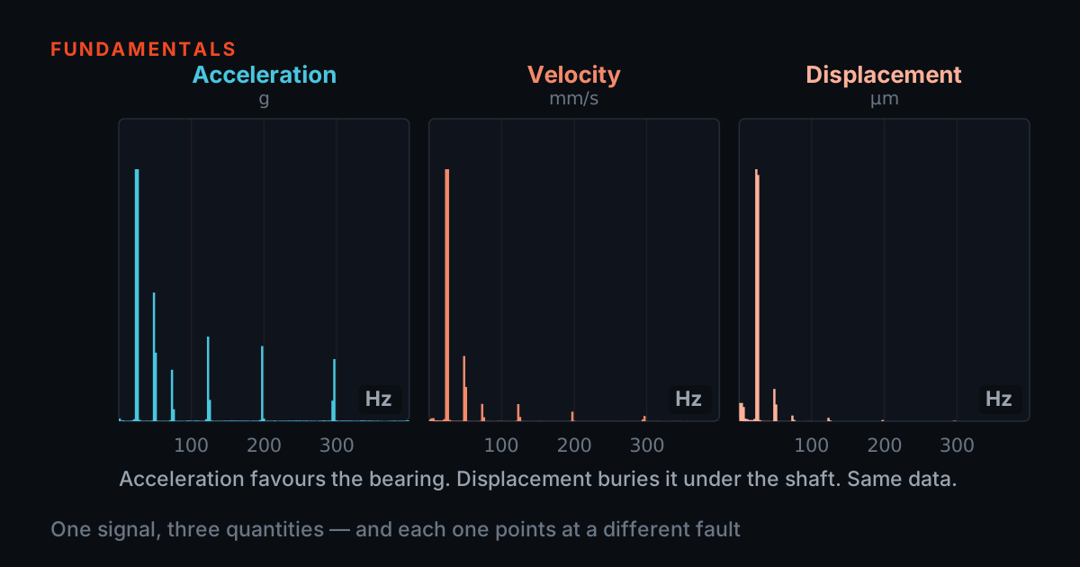
Acceleration, Velocity, Displacement: Same Motion, Three Answers — and the Traps Between Them
Two analysts measure the same bearing and report numbers that look incompatible — 0.02 g, 3 mm/s, 500 µm. All three can describe one motion, because each integration divides by frequency and tilts the whole spectrum. Here is the ω-arithmetic, the ski-slope trap that manufactures false millimetres, and how to integrate without lying.
One bearing, two analysts, three incompatible numbers
A fan bearing is surveyed twice in one week. The first analyst reports 1.9 g peak of acceleration and flags the bearing as the urgent problem. The second reports 2.1 mm/s RMS of velocity — Zone B, unrestricted operation in ISO terms — and a displacement channel on the same machine shows a startling 500 µm. Maintenance now has three verdicts for one machine: panic, relax, and condemn the foundation. Nobody has made a mistake yet. They have measured the same motion in three different quantities, and the quantities are not interchangeable numbers with different units — they weight frequency differently.
Displacement is where the metal is; velocity is how fast it is moving; acceleration is how hard it is being shaken. For a pure sine at frequency f, they are locked together: v = a ÷ (2πf) and d = v ÷ (2πf). That 2πf — ω — is the whole story of this post. It means the relationship between the three answers depends on where in the spectrum the energy sits, and it means an instrument can convert between them only by doing calculus on your signal. Calculus applied to a real, noisy, drifting signal has failure modes, and the worst of them fabricates readings that look catastrophic.
So: who is right? By the end of this post the answer will be precise — all of them can be, and one of them (the 500 µm) very likely is not, for a reason you can spot at the left-hand edge of the spectrum.
One signal, three spectra: ω is the exchange rate
- Each integration divides every spectral line by its own ω, tilting the whole spectrum by −20 dB per decade. Which peak dominates is therefore a property of the quantity displayed, not of the machine.
- Equal severity in velocity is two orders of magnitude apart in the others: 3 mm/s at 10 Hz is 48 µm and 0.019 g, while the same 3 mm/s at 1 kHz is 0.48 µm and 1.92 g.
Differentiating a sinusoid multiplies its amplitude by ω = 2πf; integrating divides by ω. Do it per spectral line and you see what that does to a whole spectrum: going from acceleration to velocity tilts everything down by a factor proportional to frequency — a slope of −20 dB per decade — and going on to displacement tilts it down again. In the other direction, differentiating tilts the spectrum up. Acceleration therefore flatters high-frequency content, displacement flatters low-frequency content, and velocity sits in between.
Put numbers on it. A component of 3 mm/s peak at 10 Hz is 48 µm of displacement but only 0.019 g of acceleration. The same 3 mm/s at 1 kHz is 0.48 µm — a hundred times less displacement — and 1.92 g, a hundred times more acceleration. Equal severity in velocity, two orders of magnitude apart in each of the other quantities. This is why a bearing tone at 2.4 kHz can tower over everything in an acceleration spectrum while being literally nanometres of displacement: 0.3 g at 2.4 kHz works out to 0.2 mm/s and 13 nm.
Both analysts in the opening were reading true spectra of the same motion. The acceleration display made the bearing tone enormous because ω² had multiplied it; the velocity display put it in proportion to the 25 Hz unbalance. Neither view is 'the real one' — they are the same information under different frequency weighting, which is exactly why you must know which weighting makes your fault visible.
Why velocity owns the severity band
- Velocity goes blind in both directions outside roughly 10 Hz to 1 kHz: low-frequency shaft position and high-frequency bearing tones both vanish from it.
- An honest 2.1 mm/s RMS overall can contain a developing bearing defect worth 0.05 mm/s. The overall answers how severe the vibration is, never whether the bearing is failing.
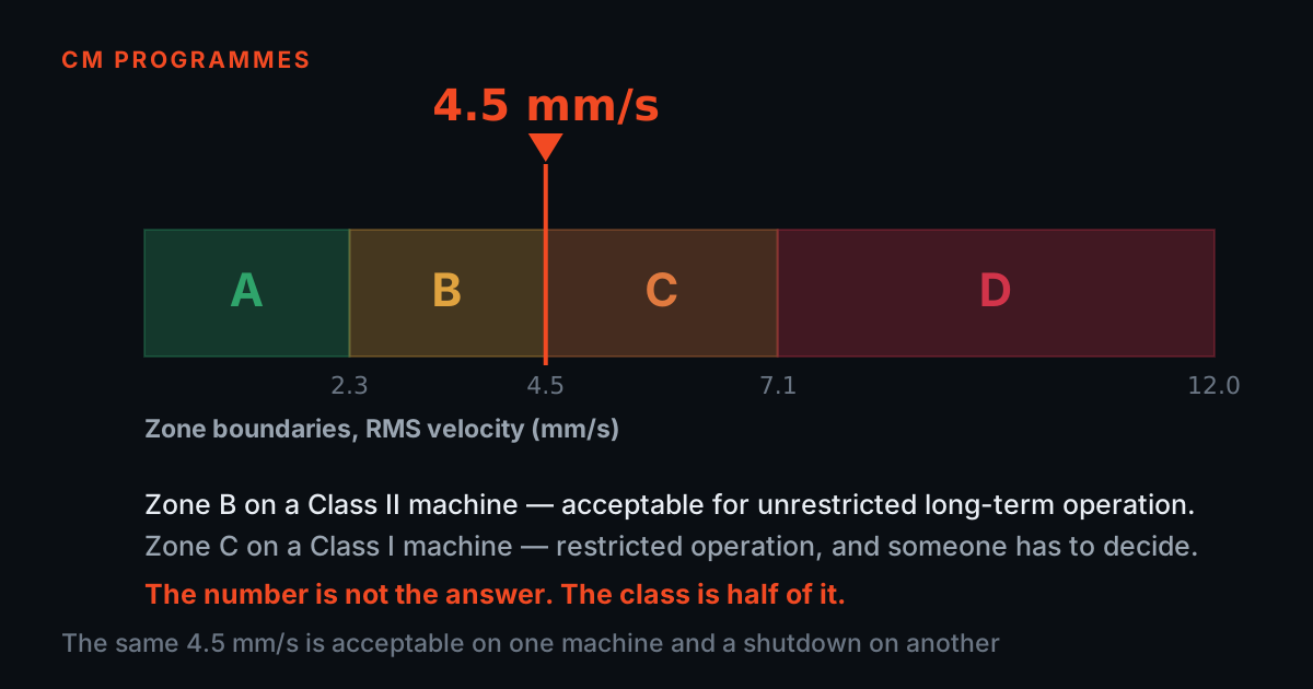
Mechanical damage correlates roughly with the energy of vibration, and across the band where most machine faults live — from a few hertz to around a kilohertz — velocity is the quantity whose amplitude tracks that energy most evenly. That is why the ISO 20816 severity zones are stated in mm/s RMS, typically evaluated over 10 Hz to 1 kHz (down to 2 Hz for low-speed machines): one number, one band, comparable across machines. Our interactive severity checker at /blog/iso-20816-severity-checker is built entirely in that quantity for that reason.
Outside that band, velocity goes blind in both directions. Below roughly 10 Hz, the faults that matter — shaft position in a fluid-film bearing, structural sway, slow-speed rolling elements — produce respectable displacement but vanishing velocity and negligible acceleration. Above a kilohertz, bearing tones, gear mesh and their harmonics produce strong acceleration but tiny velocity. A 2.1 mm/s RMS overall velocity reading can be perfectly honest and still contain a developing bearing defect worth only 0.05 mm/s — which is why bearing analysis is done in acceleration, usually with envelope processing on top.
So the second analyst's Zone B verdict answers the question 'how severe is the overall vibration?' — and answers it well. It does not answer 'is the bearing failing?'. Different quantities, different questions.
The integration trap: how nothing becomes millimetres
- Integration divides by ω, and at low frequency dividing by a small number is amplification — by ω² on the way to displacement.
- Half a milli-g of drift you cannot even see on the acceleration display reads as roughly 500 µm at 0.5 Hz. Half a millimetre, manufactured from sensor physics.
- A ski slope at the left edge of an integrated spectrum invalidates the whole reading. Re-measure once the sensor has settled before believing anything downstream of it.
Integration divides by ω — and at low frequency, ω is a small number. Dividing by a small number is amplification. Any low-frequency contamination in an acceleration signal — a DC offset from the electronics, the exponential settling of an IEPE sensor after power-up, thermal transients from bolting a cold accelerometer to a hot bearing, or the ski-slope left edge that appears below an accelerometer's low-frequency limit — gets amplified once on the way to velocity and by ω² on the way to displacement. At 0.5 Hz, dividing by ω² multiplies by about 0.1 s²: a wander of half a milli-g (0.0049 m/s²) that you cannot even see on the acceleration display reads as roughly 500 µm of displacement. Half a millimetre, manufactured from sensor physics.
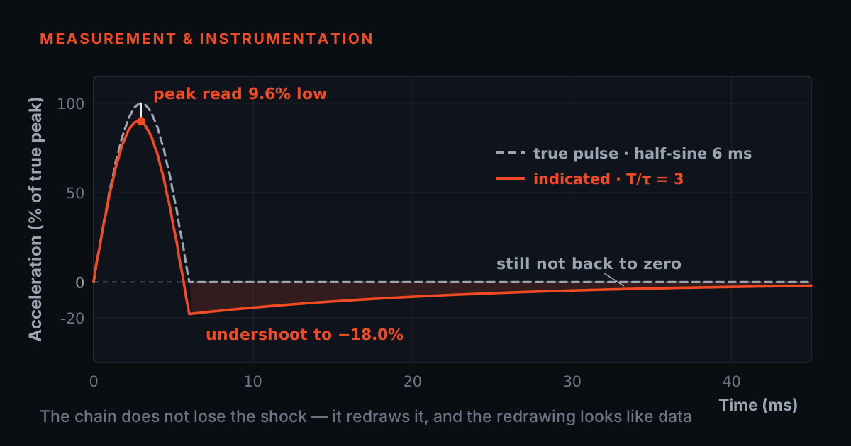
In the time domain it is even more vicious: a constant offset integrates to a ramp that grows without bound — 1 mg of offset becomes 98 mm/s of 'velocity' after ten seconds of naive integration, and 0.49 m of 'displacement'. This is why every credible instrument high-pass filters before integrating, and why the filter's corner is a specification you should know, not a detail you ignore: everything below the corner is deleted, and everything just above it is still partly amplified noise.
A representative example, not a specific customer: two readings on the same 1,485 RPM fan bearing disagree — 2.1 mm/s RMS, Zone B, from one instrument; ~500 µm pk-pk displacement, apparently catastrophic, from another taken minutes after slapping a magnet-mounted sensor onto a hot housing. The displacement spectrum shows a huge ramp at its left edge and the 'level' collapses over the next few minutes as the sensor thermally settles. The 500 µm was never motion. The rule this example teaches: a ski slope at the left edge of an integrated spectrum invalidates the whole reading — re-measure after settling, with a proper high-pass, before believing anything downstream of it.
Integrate in the frequency domain — and band-limit first
Given a sampled signal, there are two ways to integrate. Naively in the time domain — a running sum — every offset and drift error accumulates forever, which is the ramp problem above. The robust route is through the spectrum: transform to the frequency domain, divide each bin by its own jω (magnitude ÷ 2πf, phase shifted −90°), and transform back if you need a waveform. Now the integration is exact per frequency, nothing accumulates, and — critically — you can refuse to integrate where the data is garbage: zero or heavily attenuate the bins below a chosen corner before dividing, because those bins hold offset, drift and sensor roll-off, not motion.
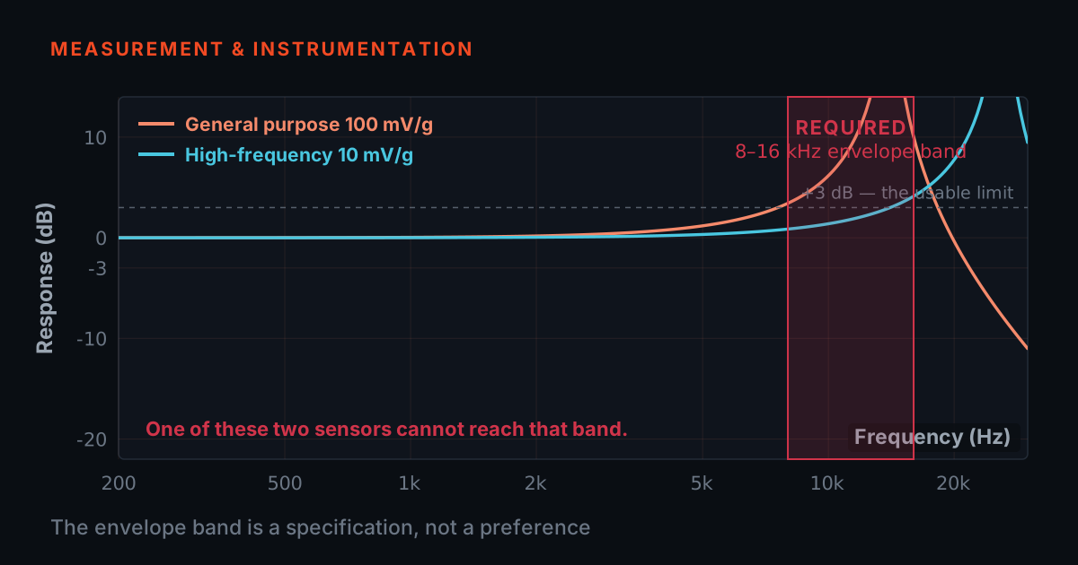
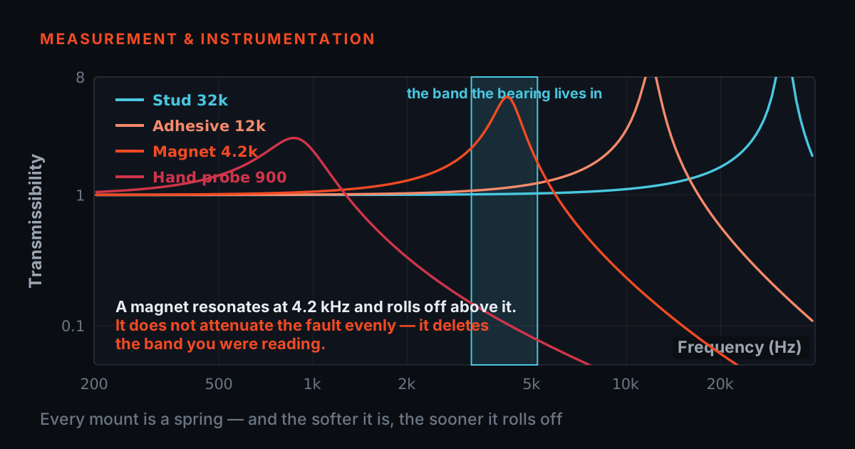
This is what a serious analyser means by 'integration': band-limited spectral integration, not a running sum. It is also why the corner frequency matters twice — once as honesty (below the accelerometer's low-frequency limit the bins are fiction anyway) and once as protection (each bin at frequency f is amplified by 1/2πf per integration, so the lowest retained bin dominates the error budget). The same logic in the other direction is why the front end matters: an alias or a mounting resonance injected at high frequency (see /blog/sample-rate-fmax-antialias and /blog/sensor-mounting-bandwidth-simulator) survives integration attenuated but present, in a band where you no longer expect artefacts.
The simulator below does the arithmetic honestly. A 25 Hz unbalance component and a 2.4 kHz bearing tone are defined in acceleration; the velocity and displacement traces are computed by dividing each spectral bin by 2πf, once and twice. Raise the bearing tone and watch it dominate acceleration while barely registering in displacement. Then switch on a small low-frequency drift — half a milli-g — and watch the displacement trace drown. The high-pass toggle shows the cure.
Units without hand-waving
- Two ladders get conflated constantly: converting mm/s to in/s is arithmetic, converting g to mm/s is calculus and needs the frequency content.
- Amplitude convention is a third, separate axis, so two honest instruments can differ by a factor of 2.8 on the same reading before any physics is involved.
- State quantity, convention, band and units — "2.1 mm/s RMS, 10 Hz–1 kHz", not "2.1".
Two different ladders get conflated constantly. The quantity ladder — g to mm/s to µm — is frequency-dependent: v = a ÷ 2πf, d = v ÷ 2πf, different at every spectral line. The unit ladder is frequency-independent bookkeeping: 1 g = 9.80665 m/s², 1 in/s = 25.4 mm/s, 1 mil = 25.4 µm. Converting mm/s to in/s is arithmetic; converting g to mm/s is calculus, and requires knowing the frequency content. An instrument that displays 'mm/s' from an accelerometer has integrated — with some high-pass corner, over some band. If you do not know that corner and band, you do not fully know what the number means.
Amplitude conventions are a third, separate axis: peak, peak-to-peak and RMS are different labels on the same quantity. For a pure sine, RMS = 0.707 × peak and pk-pk = 2 × peak — but only for a sine. A spiky bearing waveform has a crest factor far above 1.414, so 'converting' its measured RMS to peak by multiplying by 1.414 invents a number. Conventions also travel by habit: velocity severity is quoted RMS (ISO), displacement is quoted pk-pk (shaft work, because clearance is a pk-pk budget), bearing acceleration often peak or true peak. Two honest instruments can thus disagree by a factor of 2.8 on 'the same' reading — one pk-pk, one RMS — before any physics is involved.
The discipline that prevents all of this is stating readings fully: quantity, amplitude convention, band, and units — '2.1 mm/s RMS, 10 Hz–1 kHz' rather than '2.1'. Every trap in this post hides inside the words that lazy reporting leaves out.
Relative or absolute: the proximity-probe trap
There is one more way for two correct instruments to disagree, and it is not about frequency at all — it is about reference frames. An eddy-current proximity probe threads through the bearing housing and watches the shaft surface: it reports shaft displacement relative to the housing, in µm pk-pk, and it is the right tool for fluid-film machines where the danger is the shaft consuming its oil-film clearance. A seismic accelerometer bolted to that same housing reports absolute housing motion. These are different vectors: absolute shaft motion is the relative reading plus the housing motion, summed with phase.
The trap is real in both directions. On a heavy, stiff pedestal, a shaft can whirl through most of its clearance — a serious displacement problem — while transmitting so little force that the housing accelerometer reads almost nothing. On a light or resonant structure, the housing itself can move enough that the probe's 'relative' reading understates, overstates, or even phase-cancels the shaft's true absolute orbit. Comparing a probe µm number against an integrated-accelerometer µm number as if they measured the same thing is a category error, not a calibration problem.
This closes the opening puzzle properly. Acceleration, velocity and displacement from one housing-mounted sensor are one motion in three weightings — reconcilable by ω-arithmetic. A proximity probe is a different motion altogether. The complete answer to 'who is right?' is: state the quantity, the band, the convention and the reference frame, and the contradictions evaporate — except the ski slope, which was never a measurement at all. The theory behind all of this is covered step by step in TIERA's free primers at 101.tieraonline.in — free introductions, not accredited ISO certification — and for formal, assessed competence the TCAT programme is described at /services, with proctored examinations at exams.tieraonline.in.
TIERA instruments that do this work.

PhonoVibe Series — Sound & Vibration DAQ
Integration is only as honest as the low end of the chain: the 4/8/16-channel PhonoVibes are specified from 0.5 Hz, and 24-bit resolution keeps nanometre-scale bearing tones visible next to large 1× components without gain juggling.
- ADC resolution
- 24-bit, simultaneous sampling on every input
- PhonoVibe Q / O / HD
- 128 kHz · 0.5 Hz – 60 kHz · ±5 V input
- PhonoVibe D (2-ch)
- 48 kHz · 2 Hz – 20 kHz · ±10 V input
- Sensor power
- IEPE/ICP/CCLD — 24 V, 4 mA constant current, TEDS
- Calibration
- Factory calibration certificate, 1-year validity

TVIB — Sound & Vibration Analysis Software
Does exactly what this post demands: acceleration → velocity → displacement integration with FIR/IIR filtering under your control, plus harmonic, band and sideband cursors to read the result — no black-box auto mode.
- Integration
- Acceleration → velocity → displacement
- Filtering
- FIR and IIR filters, channel triggers, exp/linear/peak averaging
- FFT size
- Up to 102,400 points
- Base module
- TSAP201 — free with every PhonoVibe DAQ
- Licence
- Perpetual; 14-day fully-unlocked trial available
Sensors & Accessories
Choosing the quantity starts at the sensor: a dedicated low-frequency accelerometer for slow machinery where displacement-band content matters, a 500 mV/g industrial unit for small signals, and low-noise cabling so the left edge of your spectrum stays clean.
- Low frequency
- AC153-1D — Low Frequency Accelerometer
- High sensitivity
- 151A500D — 500 mV/g Industrial Accelerometer
- General purpose
- AC102-1D Multipurpose · AC 192-1D Compact
- Cabling
- CA-101 low-noise coaxial, 10-32 to BNC, 5 m
- Mounting
- SS304 triaxial block · magnetic mount · adhesive pads
From the TIERA store
The kit for this job
What we would actually put in front of someone doing the measurement this post describes — not the whole catalogue.
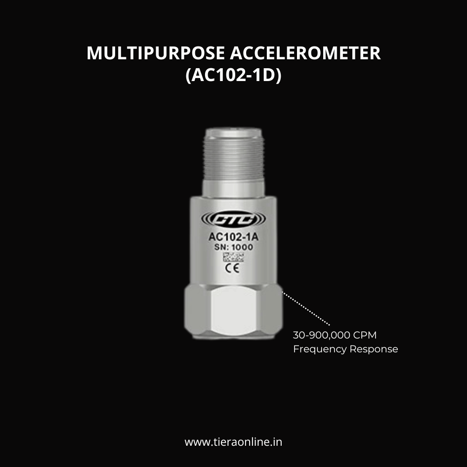 AC102-1D, MULTIPURPOSE ACCELEROMETERMULTIPURPOSE ACCELEROMETER, TOP EXIT 2 PIN CONNECTOR, 100 MV/G, ±10% 30-900,000 CPM Frequency Response (±3dB) -58 to 250 °F (-50 to 121 °C) Temperature Range Welded, Hermetic Sealing CTC’s Best Selling, Multi-Purpose Sensor Ideally Suited for Thousands of Applications₹14,750View →
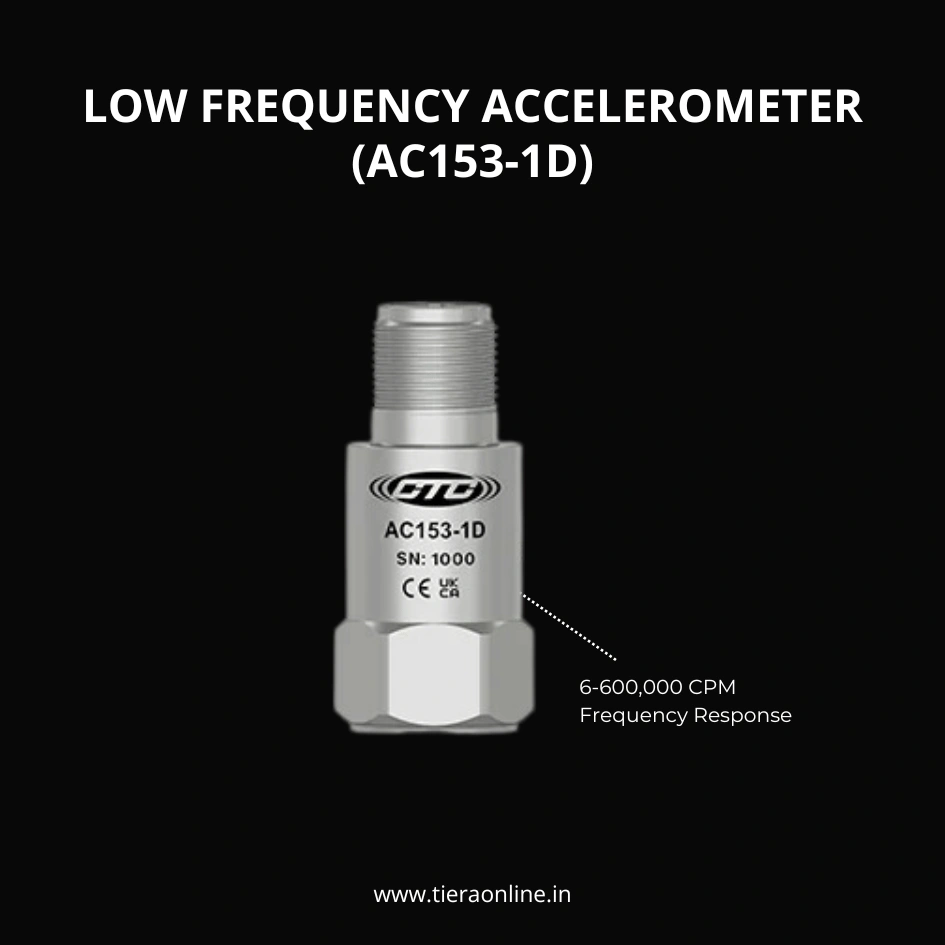 AC153-1D LOW FREQUENCY ACCELEROMETERDesigned for low speed Rotors, Main Bearings, and Gear Box Inputs, but may also be used for High Frequency Detection₹34,900View →
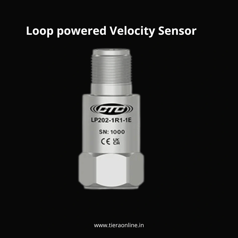 LP 202 Series, Loop powered Velocity SensorLOOP POWER SENSOR, 4-20 MA OUTPUT PROPORTIONAL TO VIBRATION IN VELOCITY, TOP EXIT 2 PIN CONNECTOR -4 to 212 °F (-20 to 100 °C) Temperature Range Welded, Hermetic Sealing 4-20 mA Current Proportional to Vibration in Velocity₹22,706View →
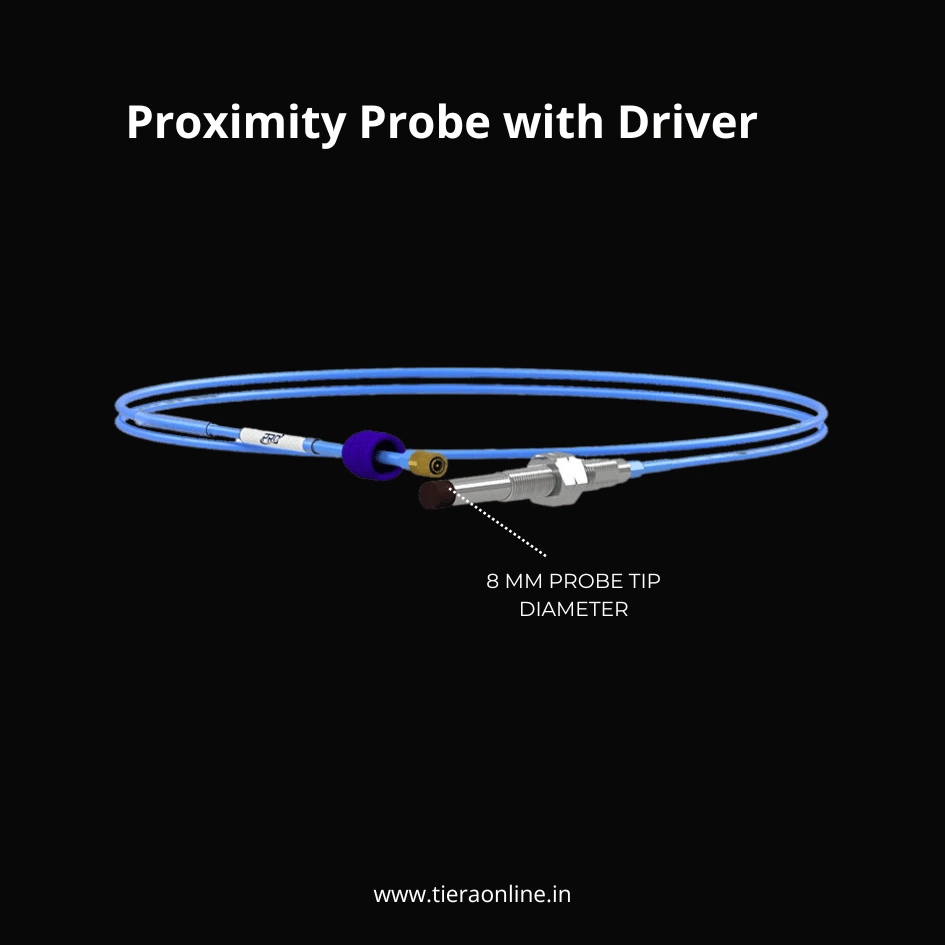 Proximity Probe with DriverPROXIMITY PROBE, 8 MM PROBE TIP DIAMETER, WITH 3/8-24 OR M10X1 CASE THREAD Measure shaft vibration and displacement on machinery with fluid film bearings. Durable PPS over-molded probe tips withstand harsh conditions when monitoring critical machinery such as turbines and compressors. Complete hardware system is compatible with all standard condition monitoring software EDDY CURRENT DRIVER COMPATIBLE WITH 8 MM PROXIMITY PROBE SYSTEMS, VOLTAGE OUTPUT API Standard 670 specified format Isolated voltage output standard at BNC and terminal block Vout and Com Upgraded to include SecureLock connector₹88,000View →
Use cases
Where this shows up in the field
Measure in the band you care about — and integrate without lying
Every trap in this post is a chain problem, and TIERA supplies the chain. Sensors matched to the band: the AC153-1D low-frequency accelerometer for slow machinery where displacement-band content lives, the 151A500D 500 mV/g industrial unit when small signals need sensitivity, compact and multipurpose IEPE options for everything between — with low-noise CA-101 coaxial cable so triboelectric noise never becomes tomorrow's ski slope. The TSP 02 and TSP 04 signal conditioners pass 0.5 Hz to 50,000 Hz at unity gain, so the low end that integration depends on survives the electronics.
The PhonoVibe DAQs specify their low-frequency limit honestly — 0.5 Hz on the 4-, 8- and 16-channel Q, O and HD, 2 Hz on the 2-channel D — with 24-bit ADCs and simultaneous sampling so a nanometre-scale bearing tone stays visible next to a large 1× line. The bundled TVIB software then does the integration the way this post argues it must be done: acceleration to velocity to displacement with FIR/IIR filtering under your control, up to 102,400-point FFTs, and harmonic, band and sideband cursors to interrogate the result in whichever quantity makes your fault visible.
- PhonoVibe Q / O / HD — 24-bit, 0.5 Hz to 60 kHz specified bandwidth: low end for integration, headroom for bearing and gear content
- TVIB acceleration → velocity → displacement integration with FIR/IIR filters — the band-limiting is yours to set, not hidden in an auto mode
- Band-matched sensors: AC153-1D low-frequency, 151A500D 500 mV/g industrial, plus low-noise CA-101 cabling and proper mounts
- TSP 02 / TSP 04 conditioners: 0.5 Hz – 50 kHz at unity gain for instruments without IEPE power
Where this sits on the TIERA learning ladder.
The theory behind this article is covered free, in full, by the TIERA 101 primers: Vibration 101 (Foundations), Accelerometer & DAQ Selection 101. They are self-paced, interactive, and end in an exam and a certificate.
The free 101 primers teach the amplitude-quantity and integration theory from first principles; the formal TCAT programme (see /services) adds structured coursework and proctored examinations at exams.tieraonline.in for teams that need assessed, certificated competence.
TIERA 101 is a free introductory primer, not an accredited ISO certification, and its hours do not count towards the formal training ISO 18436 requires.