Where the Calibration Chain Actually Begins
A comparison transfers a sensitivity; it never creates one. This is the layer beneath the traceability chain: absolute (reciprocity) calibration, which needs no reference sensor at all, and the mass-loading error that quietly biases every back-to-back comparison built on top of it. Drive the model and find the UUT mass your own tolerance can afford.
Every calibration is a comparison — until it isn't
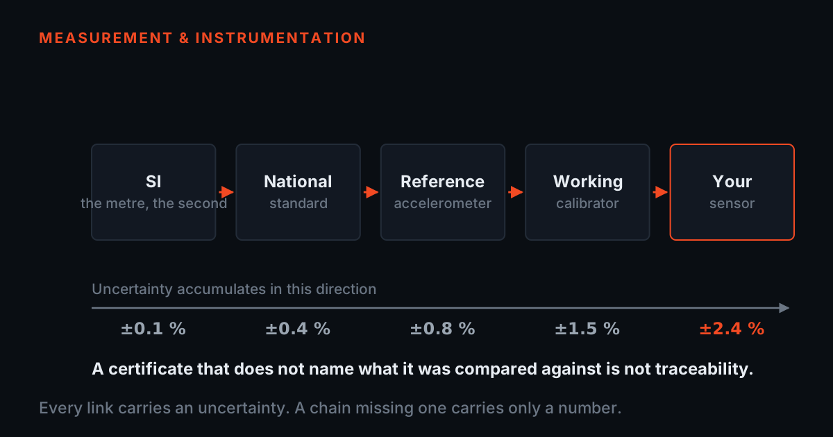
There is a companion piece to this one. /blog/calibration-traceability follows the chain of documented comparisons downwards: national standard, reference sensor with a certificate, back-to-back comparison, your sensor, your reading. It argues — correctly — that if any link is undocumented, the chain no longer reaches your number. This post is the layer directly beneath that one. It asks the two questions that post takes as given: where does the chain terminate at the top, and what is quietly wrong with every comparison hanging below it?
Start with the first. A comparison transfers a sensitivity from one device to another; it cannot manufacture one. Compare sensor B against sensor A and you learn the ratio B/A, nothing more. Compare A against a better A, and you have moved the question, not answered it. Follow that upwards far enough and either the chain closes in a circle — which proves nothing — or it terminates in a measurement that produced a sensitivity in absolute units without comparing against any pre-calibrated motion reference at all. That terminal measurement is what metrology calls a primary or absolute calibration, and reciprocity is the classic way of doing it.
Then the second question. Everything below that top link is comparison, and the workhorse comparison is back-to-back: bolt the unit under test onto a reference standard, shake both, take the ratio of their outputs. It rests on one assumption — that both sensors experience the same motion. That assumption is not quite true, it fails in a direction that is predictable, and the size of the failure depends on something nobody records: the mass of whatever you bolted on top. The second half of this post derives that error from scratch and hands you a model to drive.
Absolute calibration: a sensitivity built from mass, frequency and voltage ratios
The trick that makes reciprocity work is a property of the electrodynamic coil, not of the accelerometer. A coil in a magnetic field is a reversible electromechanical transducer: push current through it and it produces force; move it and it produces voltage. Reciprocity says those two constants are not merely related, they are the same number in SI units. The force factor in newtons per ampere and the generator constant in volts per metre-per-second are numerically identical for the same coil. That falls straight out of energy conservation — a volt-ampere is a watt, and a newton-metre-per-second is the same watt — and it is what lets an electrical measurement stand in for a mechanical one.
Now build a rig around it. Take an electrodynamic shaker whose moving assembly carries two independent coils, A and B, and mount the accelerometer standard you want to calibrate on the table. Write the total moving mass as M — table, coils, fixture, accelerometer, everything that moves together — and work at a frequency far below the moving assembly's own resonance, so the table behaves as a lumped mass and Newton's second law is the only mechanics you need. Call the two coils' constants a and b, and take three measurements.
Measurement one, the transfer admittance. Drive coil A with a current I and measure the open-circuit voltage E from coil B. Coil A produces force aI, so the table's velocity is v = aI / (jωM), and coil B generates E = bv. The ratio is therefore E/I = ab / (jωM). Repeat this with a set of accurately known masses added to the table. Because only M changes, the reciprocal of that ratio plots as a straight line against added mass: its slope gives the product ab, and its intercept gives the bare moving mass of the table. Two things you did not know are now known, from a weighing balance, a frequency and two electrical readings.
Measurement two, the voltage ratio. Still driving coil A, record simultaneously the accelerometer's output V and coil B's voltage E. The accelerometer sees acceleration jωv, so V = S(jωv), while E = bv. Their ratio R = V/E therefore equals Sjω/b — a pure number that ties the unknown sensitivity S to the unknown coil constant b.
Measurement three, the swap — this is where reciprocity earns its name. Now drive coil B instead, with current I', and read only the accelerometer. Coil B produces force bI', so the acceleration is bI'/M and the accelerometer gives V' = SbI'/M. The ratio W = V'/I' equals Sb/M, and it has the units of an impedance, volts per ampere. The same coil has just been used as a motor in one measurement and as a generator in the other, and reciprocity is the guarantee that b means the same thing in both.
Two equations, two unknowns. Multiply R by W and the coil constant cancels: RW = (Sjω/b)(Sb/M) = S(jω)S/M. Rearranged, the sensitivity is S = the square root of (M·R·W/(jω)) — in magnitude, the square root of M·R·W/ω. Check what actually went into that: a mass in kilograms, weighed; a frequency in reciprocal seconds, counted; a dimensionless voltage ratio; and a volts-per-ampere ratio. Not one of those requires a pre-calibrated vibration sensor, a reference accelerometer, or anyone else's certificate. That is what makes it primary, and that is why the chain can terminate here instead of running in a circle.
Reciprocity is not the only absolute method — laser interferometry counts optical fringes against displacement and reaches the same place by a different road, and both, along with earlier direct-viewing optical techniques, are surveyed in Endevco TP233, "Accurate Accelerometer Calibrations by Absolute and Comparison Methods". A worked step-by-step reciprocity procedure for a piezoelectric standard on an electrodynamic shaker, including the added-mass line, is documented in Endevco TP251, "Accelerometer Calibration with Reciprocity Vibration Standards". What matters for the rest of this post is not which absolute method a laboratory uses, but that one of them sits at the top, and that everything below it is a comparison.
Back-to-back comparison: what everyone downstream actually does
- S_uut = (V_uut / V_ref) × S_ref. Notice what has vanished: the absolute level of the shaking, so the shaker need not be calibrated, stable or even well behaved — drive drift divides out of the ratio.
- That robustness is why the whole industry rests on this measurement, and why nobody runs a reciprocity calibration to check a route accelerometer.
- It leaves exactly one physical premise standing: that V_uut and V_ref were produced by the same motion.
Nobody runs a reciprocity calibration to check a route accelerometer, and nobody should. The absolute measurement is slow, fussy about its assumptions and reserved for a small number of standards; those standards then transfer their sensitivity outwards by comparison, which takes minutes. The comparison of choice is back-to-back: the reference standard is a squat, stiff accelerometer with a tapped mounting surface on its top face, the unit under test screws directly into it, and both are shaken together. Endevco TP241, "Vibration Standards for Performing Comparison Calibrations", is a study of how those standards were designed for exactly this duty.
The arithmetic is one line. The reference, of known sensitivity S_ref, produces V_ref; the unit under test produces V_uut; and S_uut = (V_uut / V_ref) × S_ref. Notice what has vanished. The absolute level of the shaking never appears, so the shaker does not need to be calibrated, stable or even particularly well behaved — drift in the drive level divides out of the ratio. The frequency does not appear either, except through the sensitivities themselves. It is a beautifully robust measurement, and that robustness is why the whole industry rests on it.
The chain-of-custody half of this — what the certificate has to say, what to demand from whoever calibrates your sensors, and how a wrong stored sensitivity rescales every number in your report — is already covered in /blog/calibration-traceability, and this post does not repeat it. What that post assumes, and what the rest of this one takes apart, is the single physical premise the one-line arithmetic rests on: that V_uut and V_ref were produced by the same motion.
The assumption fails, and it fails as a velocity divider
- The reference standard is not one rigid body. Between its own crystal and its top face sits a short column of metal with real compliance, and on top of that compliance sits whatever mass you bolted on.
- Velocity divides across that series impedance exactly as voltage does: v_top / v_base = 1 / (1 − (f/f_c)²). Below the loaded resonance the mounting surface moves more than the base.
- To first order the error is (f/f_0)² × (m_u/m_c) — square in frequency, linear in the mass you attached. The reference's own crystal resonance drops out entirely.
Consider what is physically between the two sensing elements. The reference standard's own crystal is deep inside its body, referenced to the base that bolts to the shaker. The unit under test sits on the reference's top surface. Between those two places is a short column of metal — the upper part of the reference's case, its mounting boss and the stud. Metal is stiff, but it is not infinitely stiff, and above that compliance sits a mass: the top of the case plus whatever you screwed into it.
So model it as two masses on a driven base, which is the smallest model that captures the effect. Branch one is the reference's own sensing element, on its crystal stiffness, referenced to the base. Branch two is the mounting surface: an effective case mass m_c sitting on the case's axial stiffness k_c, with the unit under test's mass m_u added on top. Branch two is where the trouble is.
Work branch two in mechanical impedance, which makes it a divider and not a differential equation. For harmonic motion at angular frequency ω, the attached mass m_c + m_u presents an impedance jω(m_c + m_u) — mass impedance rises with frequency — while the case compliance presents k_c/(jω), which falls with frequency. The two are in series between the driven base and the mounting surface, and velocity divides across them exactly the way voltage divides across a series impedance. The velocity ratio between the top surface and the base is therefore [k_c/(jω)] / ([k_c/(jω)] + jω(m_c + m_u)), which tidies to k_c / (k_c − ω²(m_c + m_u)), or in the form that is easier to read: 1 / (1 − (f / f_c)²), where f_c is the resonance of the loaded mounting surface, f_c = (1/2π)·√(k_c / (m_c + m_u)). This is the same Norton-form argument that Endevco TP228, "Instrumentation for Shock and Vibration Measurements", makes generally about a transducer's own mechanical impedance disturbing the motion of whatever it is attached to; here the structure being disturbed happens to be the reference standard itself.
Read that ratio and the mechanism is obvious. Below the loaded resonance the ratio exceeds one, so the mounting surface moves MORE than the base. The unit under test therefore experiences more acceleration than the reference is reporting. The measured sensitivity, S_uut = (V_uut/V_ref)·S_ref, is inflated by exactly that ratio — you certify the sensor as more sensitive than it is, the user later divides field voltages by an inflated number, and every reading comes out low. That direction matters: the error is optimistic. It makes machines look healthier than they are, which is the failure mode nobody catches.
One more step turns this into something you can actually correct. The reference's certificate already carries its frequency response, measured bare or with a stated calibration mass, so the part of the ratio that does not depend on your unit under test is accounted for. Write the bare-case resonance as f_0 = (1/2π)·√(k_c/m_c) and let x = (f/f_0)². Then the loaded ratio is 1/(1 − x(1 + m_u/m_c)), the bare ratio is 1/(1 − x), and what the certificate cannot know — the mass-dependent residue — is their quotient:
deviation = (1 − x) / (1 − x·(1 + m_u/m_c)) − 1, with x = (f / f_0)².
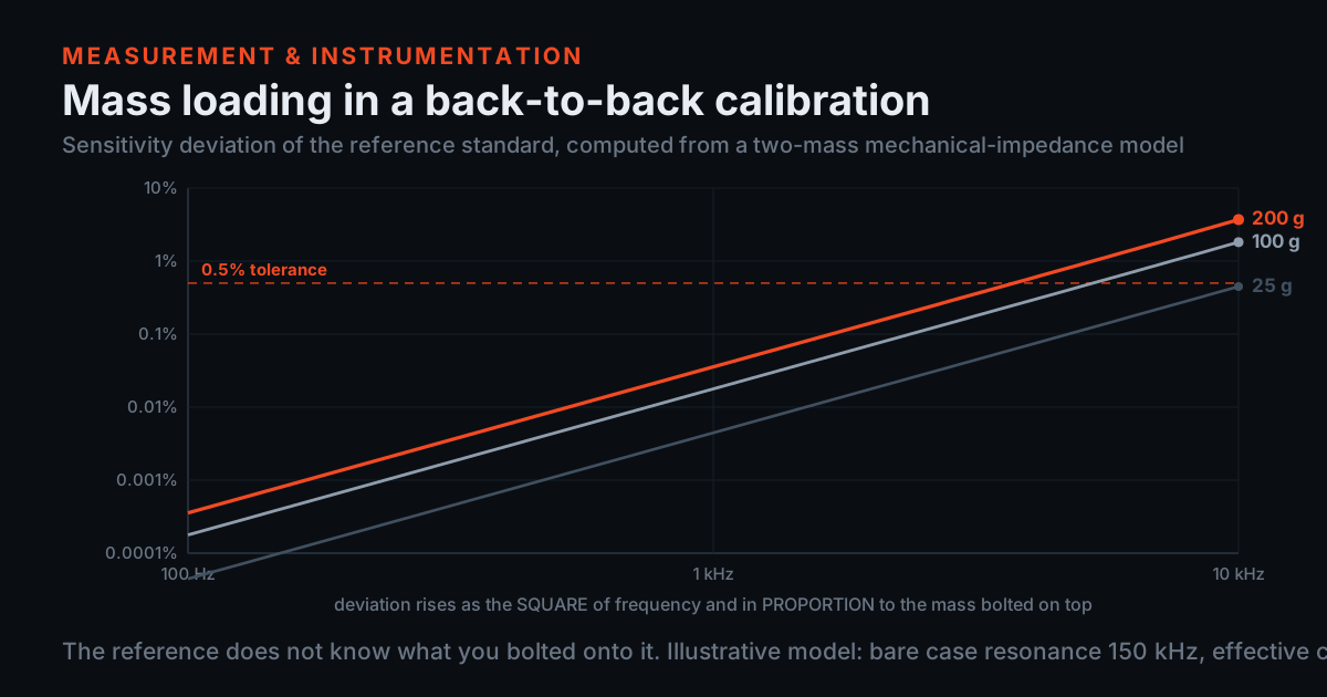
Two consequences fall straight out of that expression, and both are worth carrying around. First, expand it for small x and the leading term is simply x·(m_u/m_c) — the error grows with the SQUARE of frequency and in direct PROPORTION to the mass you bolted on. Double the frequency and the error quadruples; double the unit under test's mass and the error doubles. Second, the reference's own crystal resonance dropped out completely. It matters for the standard's frequency response, but it is on the certificate and it is the same whatever you attach; the mass-dependent bias is governed entirely by the case compliance and the mass ratio. That is the whole model, and the simulator below is nothing but this equation with two sliders on it.
The bench: find the UUT mass your tolerance can afford
The simulator below is the equation from the previous section and nothing else. Two sliders set the unit under test's mass and the frequency you care about; two selectors set your own sensitivity tolerance and how well you actually know that mass; and a switch applies the correction so you can see the size of the bias you would otherwise ship. The top panel is deviation against frequency on log axes — the square law shows up as a straight line of slope two, and every curve is parallel because mass only shifts the line up and down. The bottom panel is deviation against unit-under-test mass at the frequency you selected, with a marker where it crosses your tolerance. That marker is the number to take away: the heaviest sensor this comparison can honestly certify at that frequency.
The model parameters need to be named honestly. The bare case resonance f_0 and the effective case mass m_c are properties of a particular reference standard's mechanical design, not universal constants, so the simulator offers three illustrative values of f_0 spanning stiff to compliant and fixes m_c at 25 g. Those are teaching values chosen to put the physics in a plausible range; they are not the specification of any product, TIERA's or anyone else's. For a real standard, the manufacturer is the source — which is exactly the point Endevco TP310, "Mass Loading in Back-to-back Reference Accelerometers", makes when it argues for correcting a comparison for the mass actually attached rather than inflating the uncertainty to cover a worst-case mass range.
Three things are worth doing before you move on. Press the bench-check button and watch the deviation at 159.2 Hz collapse to 0.000451% — about four and a half parts per million — a single-point sensitivity check at the conventional reference frequency is essentially immune to this effect, which is why it is the workhorse and why this error rarely surfaces on a shop bench. Then press the frequency-response button and watch what the same rig does at 10 kHz. Then push the mass slider until the bottom panel crosses your own tolerance line, and note how much less mass that is than you expected.
Model: the two-mass mechanical-impedance divider derived above — deviation = (1 − x)/(1 − x(1 + m_u/m_c)) − 1, x = (f/f_0)². The effective case mass m_c is fixed at 25 g and f_0 is selectable. Both are ILLUSTRATIVE teaching values chosen to put the effect in a plausible range; they are not the specification of any product, and a real standard’s values come from its manufacturer. Damping is neglected, which is safe well below resonance and not safe near it. The model describes the mass-dependent residue only — the standard’s own frequency response is assumed already applied from its certificate.
What the correction buys, and what it does not
- A correction turns a large, systematic, one-directional bias into a small residual with a defensible bound. It does not turn a comparison into a primary calibration.
- What survives correction is everything the lumped model leaves out: f_0 and m_c for your particular standard, damping near the loaded resonance, stud torque and surface finish, compliance in the UUT's own base.
- The effect only bites on a frequency response running into the kilohertz — and it bites hardest for the sensors that are awkward anyway: heavy triaxials, armoured units, anything with a bulky connector.
Run the default case and the numbers make the argument on their own. At 10 kHz with a 100 g unit under test, the deviation is 1.818%: a sensor whose true sensitivity is 100.00 mV/g gets certified at 101.82 mV/g, and every field reading taken with it afterwards comes out 1.786% low. Switch the correction on with the mass known to ±5 g and that 1.818% bias becomes a ±0.0910% residual. A bias of nearly two percent has become a tenth of a percent, and the only thing that changed was arithmetic applied to a mass you could have weighed.
Now the honest half. Within this model the correction is exact when you know the mass exactly, which is precisely why the model is not the whole story. What survives correction in reality is everything the model leaves out: the uncertainty in f_0 and m_c for your particular standard, damping near the loaded resonance, a stud torque or mounting surface finish that differs from the one the standard was characterised with, and any compliance in the UUT's own base that the lumped mass does not represent. A correction turns a large, systematic, one-directional bias into a small residual with a defensible bound. It does not turn a comparison into a primary calibration.
This is also the reason to press the bench-check button. At 159.2 Hz — the conventional reference frequency for back-to-back comparison, and the one TIERA's own T-Calibro uses — the same 100 g unit under test on the same standard produces a deviation of 0.000451%. Five decimal places of nothing. A single-point sensitivity check is essentially immune to mass loading, which is why this error almost never surfaces on a maintenance bench and why the workshop practice of verifying a sensor at one reference frequency is sound. The effect only bites when the comparison is a frequency response running into the kilohertz, and it bites hardest for exactly the sensors that are hardest to handle anyway: heavy triaxials, armoured industrial units, anything with a bulky connector.
There is a practical asymmetry hiding in the square law too. Halving the frequency you certify to buys a factor of four; halving the unit under test's mass buys only a factor of two. If you have to choose where to spend effort, cap the certified bandwidth before you agonise over sensor mass. Endevco TP310, "Mass Loading in Back-to-back Reference Accelerometers", makes the complementary argument that computing the correction for the mass actually attached beats padding the uncertainty budget to cover every mass you might ever test — the two together are the whole management strategy for this error.
What to do with this on your own bench
Weigh the sensor. Not the datasheet mass — the sensor, with its mounting stud, its adaptor and whatever else travels with it into the comparison. The simulator's mass-uncertainty selector exists to show what that one act is worth: the difference between a datasheet figure and a weighing is the difference between the ±0.0910% residual the simulator prints on its defaults and a smaller one, at the cost of thirty seconds on a balance you already own.
Read the reference standard's own documentation for its mass-loading behaviour, and if it is not stated, ask. A standard characterised with a stated calibration mass, or supplied with correction data as a function of attached mass, lets you compute; a standard supplied with neither leaves you inflating an uncertainty to cover the worst case, which is the outcome this whole post exists to avoid.
Separate the two jobs your calibration does. A single-frequency sensitivity check — the one that catches the dropped sensor, the drifted one, the one that quietly disagrees with its neighbours — belongs at a reference frequency where this effect is five decimal places of nothing, and should be done often. A frequency-response calibration into the kilohertz is a different exercise with different error sources, and it is the one that needs the correction, the mass on the certificate, and a stated bandwidth limit.
Then put the number back in context. A 1.8% mass-loading bias is real, but /blog/calibration-traceability makes the case that a sensor nobody has compared against anything in three years is a far larger risk, and /blog/daq-quality-and-testing shows how much of a measurement can be lost between the sensor and the file regardless of how well the sensor was calibrated. If you are choosing where to spend attention: verify often at one frequency first, correct for mass second, and buy uncertainty budget last.
One closing note on what this post is not. It is a derivation and a model, published so the physics is inspectable — every number above is reproducible by driving the simulator with the stated parameters. It is not a metrological service description, and nothing here should be read as a statement about accreditation, scope or measurement uncertainty for any laboratory, TIERA's included.
TIERA instruments that do this work.

T-Calibro Vibration Calibration System
The comparison side of everything above, on a bench: back-to-back at a single reference frequency, where mass loading is a few parts per million and a drifted sensor is not.
- Method
- Back-to-back comparison calibration method
- Calibration frequency
- Standard reference at 159.2 Hz (≈1000 rad/s), per ISO 16063 back-to-back convention
- Compatibility
- Compatible with all IEPE/ICP accelerometers
- Design
- Portable bench-top design — no external signal generator required
- Records
- T-Calibro software: automated calibration record and certificate generation

TVIB — Sound & Vibration Analysis Software
A sensitivity is only useful once it is entered somewhere. TVIB scales each channel independently, so a corrected sensitivity goes in per sensor rather than as one global fudge.
- Base module
- TSAP201 — free with PhonoVibe
- Scaling
- Up to 102,400-point FFT, multi-channel scaling, independent calibration
- Analysis
- Time waveform + narrowband FFT, harmonic / band / sideband cursors
- Integration
- Integration for acceleration → velocity → displacement
- Licence type
- Perpetual; free updates for 2 years, AMC after
From the TIERA store
The kit for this job
What we would actually put in front of someone doing the measurement this post describes — not the whole catalogue.
 T-Calibro _ Precision Sensor Calibration Device for Accelerometers & Vibration SensorsT-Calibro is a high-performance PC-based vibration calibrator designed to calibrate and verify the working conditions of accelerometers, velocity sensors, and vibration meters. It provides stable, traceable vibration signals and supports IEPE, charge and voltage-type sensors, ensuring complete flexibility for industrial, laboratory, and R&D environments.₹18,00,000View →
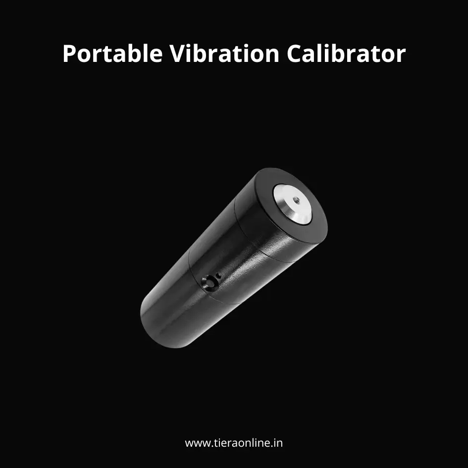 VC 01- Portable Vibration CalibratorVibration Calibrator Rapid judgement of measurement system integrity. Rapid measurement of the Sensitivity of the Acceleration/ Velocity/Displacement sensors. Battery powered with automatic shutdown. Self-contained vibration reference. Small size. Light weight₹1,41,000View →
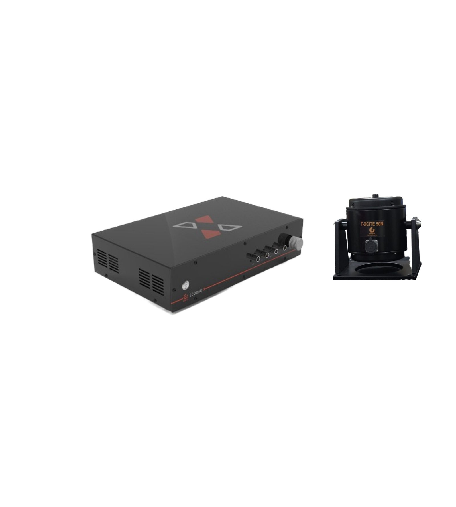 TXcite 50 – Electrodynamic Shaker (50 N) with AmplifierT-Xcite Permanent magnet modal shakers provide precise, reliable, stable and long-lasting operation. Highest quality materials, stringent quality control and rugged construction General mechanical mobility measurements Experimental modal analysis on most mechanical structures SISO, MISO. SIMO and MIMO modal test applications Advanced structural dynamics investigations Structural damage detection Finite element model correlation₹4,80,000View →
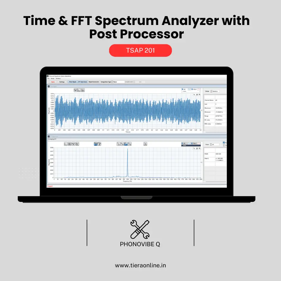 TSAP 201 -Time & FFT Spectrum Analyzer with Post Processor (Phonovibe Q)Use Cases Bump Test Product Development Off route Machine Vibration analysis. Drop Test Product Development & Research₹34,560View →
Use cases
Where this shows up in the field
- Wireless Sensor Validation LabWireless sensor / accelerometer OEM running validation labs See the setup →
- End-of-Line Quality TestingOEM production line — automotive driveshafts, pumps, motors See the setup →
- Modal Analysis and Structural Dynamics R&DMechanical R&D / structural dynamics lab See the setup →
Verify often at one frequency; correct deliberately at the rest
The argument this post makes is that the two jobs a calibration does are different jobs. The one that catches real trouble — the dropped sensor, the slow drifter, the unit that quietly disagrees with its neighbours — is a single-point sensitivity check at a reference frequency, and it should be routine rather than annual. The T-Calibro is built for exactly that: back-to-back comparison at a standard reference of 159.2 Hz, compatible with all IEPE/ICP accelerometers, on a portable bench-top design that needs no external signal generator, with software that generates the calibration record and certificate automatically.
The second job — a frequency response running into the kilohertz — is where the mass-loading model above earns its keep, and where the number you need is the reference standard's own case behaviour and the weighed mass of the sensor in front of you. Whatever you conclude, the corrected sensitivity has to land in the software channel by channel: TVIB scales and calibrates each channel independently, so a per-sensor number stays a per-sensor number.
- T-Calibro — back-to-back comparison calibration method, compatible with all IEPE/ICP accelerometers
- Standard reference at 159.2 Hz (≈1000 rad/s), per ISO 16063 back-to-back convention — the regime where mass loading is negligible
- Portable bench-top design, no external signal generator required; factory calibration certificate included with unit
- TVIB — independent per-channel calibration and scaling, so a corrected sensitivity is entered where it belongs
Where this sits on the TIERA learning ladder.
The theory behind this article is covered free, in full, by the TIERA 101 primers: Accelerometer & DAQ Selection 101, Measurement Setup 101. They are self-paced, interactive, and end in an exam and a certificate.
The primers cover what sensitivity is and how a measurement chain is set up; this post sits above them, at the point where a sensitivity is created rather than used. TCAT adds examined depth on calibration practice and on reasoning about measurement error — the free primers explain; TCAT verifies.
TIERA 101 is a free introductory primer, not an accredited ISO certification, and its hours do not count towards the formal training ISO 18436 requires.