Published · Updated
Planning Wireless Gateway Coverage: Range, Walls and Sensors per Gateway
A line-of-sight range figure is not a plant range figure, and mistaking one for the other is the most expensive error in wireless condition-monitoring procurement. A stated path-loss model you can drive, so you can watch how fast steel and distance eat a link budget — and a straight answer on how many sensors one gateway really carries.
A line-of-sight range figure is not a plant range figure
- A line-of-sight range is measured across a car park with nothing between the antennas — no floor, no walls, no forklifts.
- The gap between that and a plant is routinely a factor of five to ten in distance, which is twenty-five to a hundred in the area one gateway covers.
- The answer to a coverage shortfall is almost always more gateways, closer — not a bigger antenna or a longer-range sensor.
Every wireless sensor datasheet carries a range. The CTC ConnectSens families quote 1,200 ft — 366 m — for the dynamic nodes and 2,100 ft — 640 m — for the overall node, as recorded in TIERA's technical brief on the range. Those are honest figures and they are clearly labelled LINE OF SIGHT. The trouble starts one step later, when somebody opens a plant drawing, scales off eighty metres from the proposed gateway position to the furthest pump, sees that eighty is comfortably less than 366, and signs the order.
Line of sight means what it says: nothing between the two antennas, no floor, no ceiling, no walls to reflect from, no forklifts. It is a number measured across a car park. What a plant does to 2.4 GHz is a completely different problem, and the gap between the two is not ten or twenty per cent. It is routinely a factor of five to ten in distance, which is a factor of twenty-five to a hundred in the area one gateway covers.
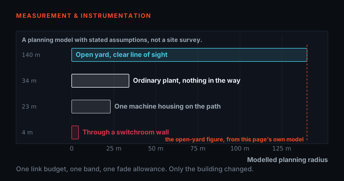
The table below is that gap, computed. Every row uses exactly the same link budget — the same node, the same antenna, the same level the gateway needs, the same fade allowance. Only the building changes. The open-yard figure is 140 m; an ordinary plant floor with nothing at all in the way is 34 m; put one machine housing on the path and it is 23 m; ask it to go through a switchroom wall and it is 4 m.
One thing about that first row has to be said out loud, because it looks like more than it is. The gateway's own store page publishes a "Connected Sensor Range" of ≥ 140 m — and the open-yard row of the table below also comes out at 140 m. That is a coincidence of the inputs, not a derivation of the specification, and we would rather point at it than let you find it and draw the wrong conclusion.
Here is why it is a coincidence. We picked the fade allowance ourselves. We assumed the sensor's own internal antenna. What we did put in were two published figures — the gateway's −75.0 dBm supported floor and its 6 dBi antenna — and free-space physics, which is not judgement at all. Feed those in and 140 m is simply what falls out. It is worth knowing, because it means our model and the manufacturer are describing the same radio rather than two different ones. It is NOT evidence that this model is right about anything else on this page, and it is no evidence whatsoever for the plant exponents in the rows beneath it. Those are TIERA's engineering judgement and nothing more.
And be clear about what the manufacturer's figure is not. It is labelled "Connected Sensor Range", it carries a dagger footnote whose text we do not have, and it does not say line of sight anywhere. The genuine line-of-sight figures in this range are the 640 m and 366 m quoted at the top of this section, and those belong to the SENSORS, not to the gateway. Anyone who reads the gateway's 140 m as a line-of-sight figure, or reads this table's first row as confirming it, has made exactly the mistake this post exists to prevent.
None of this means the datasheet lied or that wireless does not work. It means the coverage question has to be answered with a link budget rather than with a tape measure, and that the answer is almost always MORE GATEWAYS, CLOSER, rather than a bigger antenna or a longer-range sensor. The rest of this post derives that, hands you the model, and then tells you what to do with it.
One link budget, six environments. Every row uses the same 10 dBm node, the same 2 dBi internal antenna, the same 6 dBi gateway antenna, the same −75.0 dBm supported floor and the same 10 dB fade allowance. Only the building changes. The exponents and the obstruction figures are TIERA field guidance for planning, not measurements; the radii are computed from them by the same function the bench below runs.
| Environment | Exponent | Obstruction | Planning radius | Of the open-yard figure |
|---|---|---|---|---|
| Open yard, clear line of sight the brochure condition, and the only one that is physics rather than judgement |
n = 2.0 | 0 dB | 140 m | 100% |
| Light plant, spaced machines an open roof and little overhead steel |
n = 2.5 | 0 dB | 52 m | 37% |
| Ordinary plant, clear path nothing between the two, but a built environment around them |
n = 2.8 | 0 dB | 34 m | 24% |
| Ordinary plant, one machine housing on the path the gateway is at working height, among the machines |
n = 2.8 | 5 dB | 23 m | 16% |
| Congested plant, mezzanine grating between the gateway is on the wrong deck |
n = 3.0 | 15 dB | 9 m | 6% |
| Congested plant, switchroom wall between RCC and a steel door - the single most common planning mistake |
n = 3.0 | 25 dB | 4 m | 3% |
Where the decibels go
A link budget is addition and subtraction, and there are only five terms in it. The node transmits at some power. Its own antenna adds a little gain, or costs a little. The path takes a large amount away. The gateway's antenna adds some back. What arrives has to be above the level the gateway needs, with something left over. That leftover is the LINK MARGIN, and it is the only number in wireless planning worth arguing about.
The path term is where the interesting behaviour lives, and it splits into three. First there is the loss in the first metre, which at 2400 MHz is 40.1 dB. That is a constant of the band. It is not something a plant does to you and it is not something you can buy your way out of; it is the price of using 2.4 GHz at all, and it is why the figure below starts with a large grey block that nobody can shrink.
Second there is spreading beyond that first metre, and this is the term the plant governs. In free space it costs 20 dB per decade of distance — 6.0 dB every time you double the distance. In a built environment it costs 10 × n dB per decade, where n is the path-loss exponent: reflections, absorption and diffraction all take their cut, and n rises. Between free space at n = 2.0 and an ordinary plant at n = 2.8, the same 100 m hop costs 16.0 dB more. Nothing is in the way in either case.
Third there is whatever is actually in the way, which is added on top as a flat penalty. A wall is a wall wherever it stands. And this is the fact that makes coverage planning counter-intuitive: because the exponent multiplies DECADES of distance, the same wall is affordable on a short hop and ruinous on a long one. It is not that the wall changed. It is that on a long hop there was nothing left to spend.
The figure below is one case, itemised: 40 m across an ordinary plant floor at n = 2.8, with 5 dB of plant steel on the path — which is the bench's own starting position, so the numbers you see here are the numbers you will see when you scroll down. It lands at −71.9 dBm against a −75.0 dBm floor: a margin of 3.1 dB, which closes the link and does not cover the fade allowance. That is a link that works on the day it is commissioned.
What a plant does to 2.4 GHz
Ask what a wall costs and you will get a range, because it genuinely depends on the wall — its thickness, its water content, what reinforcement is in it, whether the path goes through it square-on or at a grazing angle, and how much of the signal is arriving by a reflected path that misses the wall entirely. Anybody who gives you a single confident number for a brick wall is telling you about their spreadsheet, not about your plant.
What is still useful is a planning bracket: a set of figures that are the right order of magnitude, that let you rank one gateway position against another, and that are honest about being judgement. The table below is TIERA's. It is engineering judgement from installing and supporting instrumentation in Indian industry, and it is aimed squarely at what Indian industrial construction actually uses — 115 mm and 230 mm brick, cast RCC, and steel-doored switchrooms. Nobody measured these walls. They are a starting point for deciding where to stand with a real radio, and they are not a substitute for standing there.
The two families in it behave differently in practice, which is why they are separate sliders on the bench. Building fabric is usually not negotiable: the wall is where the wall is, and your options are to route around it or to put a gateway on both sides. Plant steel very often IS negotiable, because it is a consequence of where the gateway was mounted — and gateways get mounted at working height, among the machines, because that is where somebody found a socket and a network point. A gateway two metres higher, above the skids rather than between them, frequently gains more than any antenna in the catalogue.
The steel case worth dwelling on is the last row: a sensor inside a metal enclosure. Thirty decibels is a factor of a thousand in power, and it turns a 34 m planning radius into 3 m. This comes up constantly with sensors mounted inside machine guarding or terminal boxes, and it is the one case where moving the gateway closer is the WRONG answer — the problem is not the length of the path, it is what is wrapped around one end of it. The bench flags that case explicitly, because the fix is different.
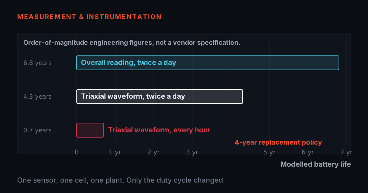
One more thing the table cannot show you, and it matters for a wireless CM programme specifically: a marginal link is not a free one. A node at the edge of its range re-sends packets, and every re-send comes out of the same primary cell that has to last four years. That is why published battery-life figures carry "with excellent signal strength" in their own fine print, and it is why coverage planning and battery planning are the same conversation. TIERA's post on wireless battery life prices that in joules; this one prices it in decibels.
TIERA field guidance for planning. Not measurements. These are the figures TIERA plans Indian plant installations with, and they are engineering judgement about 2.4 GHz through the building fabric and the plant steel that Indian industrial construction actually uses. Nobody measured these walls. The radius column is what each one does to the 34 m an ordinary plant gives on a clear path at n = 2.8, computed by the same function the bench below runs. Use this to decide where to stand with a real radio, never instead of one.
| What is on the path | Kind | Planning figure | Radius at n = 2.8 | Where it comes up |
|---|---|---|---|---|
| a light partition | Building fabric | 4 dB | 25 m · 72% | plasterboard, ply, or a glazed office wall |
| a 115 mm brick wall | Building fabric | 6 dB | 21 m · 61% | a half-brick plant partition |
| a 230 mm brick wall | Building fabric | 12 dB | 13 m · 37% | a full-brick external or bay-dividing wall |
| a 150 mm RCC wall or floor slab | Building fabric | 18 dB | 8 m · 23% | cast concrete with reinforcement in it |
| a switchroom or DG-room wall | Building fabric | 25 dB | 4 m · 13% | RCC with a steel door in it - the classic mistake |
| one motor or pump housing | Plant steel | 5 dB | 23 m · 66% | a single cast body directly on the path |
| a machine skid or guard | Plant steel | 8 dB | 18 m · 52% | a fabricated frame and sheet guarding |
| a bank of control panels | Plant steel | 12 dB | 13 m · 37% | sheet-steel cubicles in a row |
| a steel grating mezzanine floor | Plant steel | 15 dB | 10 m · 29% | the gateway is on the wrong deck |
| cable trays plus structural steel | Plant steel | 20 dB | 7 m · 19% | a congested overhead run the whole way |
| inside a steel enclosure | Plant steel | 30 dB | 3 m · 8% | the sensor or the gateway is in a metal box |
Sketch your own coverage
Here is the bench. Seven controls, a plan view with the computed coverage radius drawn on it, and the link budget itemised underneath. Click anywhere on the plan to drop the sensor at that distance — it snaps to the nearest step, so the drawing and the slider always agree. The chips along the top load the cases this post discusses, so you can reproduce every figure above rather than taking it on trust.
Watch the itemised budget rather than the margin. The margin tells you whether this position works; the split tells you what to change if it does not. If spreading is the big term, the lever is a shorter hop, and the arithmetic is brutally simple: halving the distance buys you 3 × n decibels, which at an ordinary plant's exponent is about eight and a half — more than any antenna on the price list. If obstructions are the big term, distance is not your problem and shortening the hop is wasted effort.
Four of the chips are deliberate failures, and they fail for four different reasons. The plant chip fails with NOTHING in the way, purely from the exponent. The switchroom chip fails because of what is in the way. The bigger-antenna chip fails to fix the switchroom chip, which is the point of it — 2 more decibels of antenna against a 20.1 dB deficit changes the number and not the answer. And the cabinet chip fails at 10 m, closer than any other failure on the bench, because the sensor is in a metal box. A coverage tool that only ever says yes is a sales tool.
The chip that fixes the switchroom is the last one, and it is not hardware. Same node, same power, same antenna, same congested plant — the gateway simply moves to the same side of the wall as the machines it serves, 15 m from them, and the margin goes from -20.1 dB to +17.7 dB. That is the whole of coverage planning in two clicks.
- Path loss, itemised
- —
- Level at the gateway
- —
- Link margin
- —
- Planning radius
- —
This is a planning model with stated assumptions, not a site survey, and it is four lines: the loss at one metre is 20 log₁₀(f in MHz) − 27.55, which is 40.1 dB at 2400 MHz; beyond a metre the path costs a further 10 × n × log₁₀(d); obstructions add a flat penalty in decibels; and the margin is the transmit power plus both antenna gains, less the path loss, less the level the gateway needs. Those lines are the same source text the unit tests for this page run against. Traceable to a manufacturer, from files in this repository: 2400 MHz and Bluetooth Low Energy 5.2, the −75.0 dBm bottom of the published −20 to −75 dBm supported signal-strength window, and the 140 m connected-sensor range, all from the Access2000 gateway store page — and note that this bench’s free-space answer landing on that same 140 m is a coincidence of the inputs, set out in the first section of this post, not a derivation of the manufacturer’s figure and not a line-of-sight claim; and 6 dBi of 360° omnidirectional gain, with two antennas required per gateway, from the antenna store page. TIERA's engineering judgement, not anybody's datasheet: every path-loss exponent, every obstruction figure in decibels, the 2 dBi assumed for the sensor's internal antenna, the transmit-power ladder, the sensitivity rungs below the published floor, and the 10 dB fade allowance. Take the real figures for a part you are buying from its own datasheet, and take the real path loss from a radio walked around your own plant.
How many sensors per gateway matters less than you think
- Throughput is not the ceiling and never was — ask instead about concurrency: how many radio connections a gateway holds open at once, which is a much smaller number than how many sensors it can register.
- Coverage binds long before any sensor count does. A gateway rated for thirty sensors only helps thirty sensors inside its planning radius, and on a real layout that is often five or eight.
- The retry loop connects the two: an edge sensor re-sends, holds its slot longer, delays everyone else and drains its own battery — fleet behaviour degrades from the edges inward.
- The specification worth asking for is points per gateway inside a stated planning radius, with a stated fade allowance, at a stated cadence.
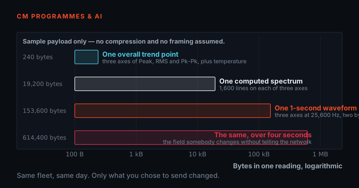
The second question every wireless buyer asks is how many sensors one gateway carries, and it is usually asked as though the answer were about bandwidth. It is not, and the arithmetic settles it in one line. A full triaxial waveform at the largest record these nodes offer is 153,664 bytes. At a delivered application throughput of 250 kbit/s — TIERA's engineering judgement of what a Bluetooth Low Energy link actually achieves once protocol overhead and connection intervals are paid for, not a nameplate symbol rate — that is 4.9 seconds of radio time. At 2 readings a day, each sensor asks for 9.8 seconds of the day.
The Access2000 gateway's store page publishes 30 sensor inputs. Thirty sensors at that duty cycle is 295 seconds — 4.9 minutes — out of 86,400. That is 0.34 per cent of the day. Throughput is not the ceiling and it never was, which is why arguing about sensor counts as though they were a bandwidth problem misses the actual constraints.
There are three real ones. The first is CONCURRENCY, not capacity: a gateway can hold a certain number of radio connections open at the same moment, which is a different and much smaller number than how many sensors it can have registered. Exceeding it does not break anything — the readings queue and arrive later. It stretches the window in which a fleet reports, and if your analysis depends on readings across a train being roughly simultaneous, that stretch is the thing to ask about. Ask the manufacturer for the concurrent figure and the queueing behaviour above it, in writing, and do not accept the registered-sensor count as an answer to it.
The second is COVERAGE, which is this whole post, and it binds long before any count does. A gateway rated for thirty sensors is only useful for thirty sensors that are inside its planning radius. In an ordinary plant that radius is tens of metres, not hundreds, so the practical limit on sensors per gateway is usually how many measurement points sit inside a circle that small — and on a real plant layout that is often five or eight, not thirty.
The third is the RETRY LOOP, and it connects the two. A sensor at the edge of coverage re-sends, which lengthens its airtime, which occupies a connection slot for longer, which delays other sensors, which pushes the reporting window wider still — and it drains that node's battery faster than any of its neighbours. Fleet behaviour degrades from the edges inward. This is the mechanism behind the classic complaint that a wireless system "worked at commissioning and got worse", and it is a coverage problem wearing a capacity problem's clothes.
So the useful specification is not sensors per gateway. It is points per gateway INSIDE A STATED PLANNING RADIUS, with a stated fade allowance, at a stated cadence — and if a supplier will quote you that, they have done the work.
Placement patterns that work
High and central beats powerful and remote, every time. The single highest-value move in wireless CM installation is to get the gateway above the machines rather than among them: it removes the plant-steel term almost entirely, and on the ladder in this post that term is worth up to 30 dB. Mount it in the middle of the area it serves rather than at one end, because coverage is a radius and putting the gateway in a corner throws away three quarters of it.
That is what the antennas are for, and it is worth being precise about what they do and do not buy. The published omnidirectional antenna gives 6 dBi of 360-degree coverage, and the antenna page notes that two are required per gateway. Six decibels is real and worth having — it is roughly the difference between 34 m and 21 m of planning radius at n = 2.8. But it is a few decibels against obstruction terms that run to twenty-five and thirty, and it is omnidirectional gain, which comes from flattening the pattern vertically. On a gateway mounted high above a floor of sensors, that flattening is not always your friend.
Power the gateway where it needs to be, not where the power is. This sounds obvious and it is the reason more gateways end up in switchrooms than anywhere else: the network point and the socket are both in there, so that is where the box goes, and the RCC wall and the steel door are then between the gateway and every sensor it serves. Power over Ethernet is the answer to this and it is worth designing around from the start — the gateway takes PoE, an injector puts PoE onto an ordinary run where the switch cannot, and the position then follows the radio rather than the electrics.
Overlap deliberately rather than tiling. Two gateways whose planning circles touch will both see the sensors in the overlap and can share them; two gateways whose circles merely abut leave a seam where every sensor is marginal, and marginal sensors are the ones that drain batteries and stretch reporting windows. Plan for the circles to overlap by something like a third of a radius, and put the seams where there are no measurement points rather than through the middle of a machine train.
And survey. Everything on this page is a planning model with stated assumptions; it is deliberately not a site survey and the canvas says so on its face. What it is for is deciding where to stand with a real radio and how many positions to try — which turns a survey from a day of wandering into an afternoon of checking four candidate positions. Walk the plant with a gateway and one sensor, read the actual received level at each proposed point, and believe that reading over anything in this post. The model's job is to make the survey short, not to replace it.
- Mount the gateway above the machines rather than among them, which removes almost all of the plant-steel term.
- Put it in the middle of the area it serves, because coverage is a radius.
- Run Power over Ethernet so the position follows the radio rather than the electrics.
- Overlap adjacent planning circles by something like a third of a radius, and put the seams where there are no measurement points.
- Walk the plant with a real gateway and sensor and believe the received level you read over anything modelled.
- Do not mount at working height among the skids because that is where the socket is.
- Do not put the gateway in a corner of the area it serves.
- Do not put it in the switchroom and leave an RCC wall and a steel door between it and every sensor.
- Do not tile coverage circles edge to edge — the seam is where sensors go marginal and batteries drain.
- Do not buy antenna gain to fix an obstruction problem; a few decibels does not answer twenty-five.
What to ask a supplier
- The two answers that matter most are whether the quoted range is line of sight, and what received level the gateway needs for supported operation as distinct from raw receiver sensitivity — those two are typically twenty decibels apart.
- A supplier who will bring a gateway and a sensor and walk your points before quoting has done the work. One who quotes a sensor count from a floor area has not.
- Settle the coverage question before the sensor question: gateway positions drive the network and power runs, which is the part with the lead time.
Six questions turn a coverage claim into something checkable. Ask them in writing and the conversation stops being about brochure ranges.
First: is that range figure line of sight, and what path-loss exponent would you plan our building with? Second: what received level does the gateway need for supported operation, as distinct from the raw sensitivity of its receiver — those two are typically twenty decibels apart and only one of them is a promise. Third: how many concurrent radio connections, as distinct from registered sensors, and what happens to the reporting window above that number? Fourth: what does the antenna's pattern look like vertically, given we intend to mount the gateway six metres above a floor of sensors? Fifth: does the gateway or the software report a per-sensor received level, so we can find marginal points before they become battery problems? Sixth: what is the recommended overlap between adjacent gateways?
Then ask for the thing that actually settles it, which is a survey. A supplier who will bring a gateway and a sensor to your plant and walk your points before quoting is a supplier who intends the installation to work. One who will quote a sensor count from a floor area has not done the arithmetic on this page, and the gap will surface at commissioning at your expense rather than theirs.
And decide the coverage question before the sensor question, not after. Where the gateways go determines how many you need, which determines the network and power runs, which is the part of a wireless CM programme that involves other departments and therefore the part with the lead time. The sensors are the easy bit.
TIERA instruments that do this work.
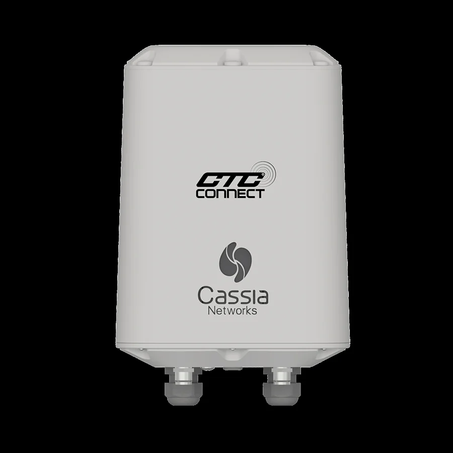
Access2000 Series — Long-Range Wireless Gateway & Network Controller
The box every number on this page is planned around. Two of its published specs are the ones coverage planning actually turns on, and it is worth reading them together: a connected-sensor range of at least 140 m, and a SUPPORTED signal-strength window of −20 dBm to −75 dBm. The second is the useful one, because it is a supported-operation figure rather than a raw receiver sensitivity — it already has the manufacturer's own margin in it, which is exactly what you want to plan against.
- Connected Sensor Range
- ≥ 140 m†
- Supported Signal Strength
- -20 dBm to -75 dBm†
- Sensor Communication
- Bluetooth ® Low Energy 5.2 from CTC ConnectSens
- Input Count
- 30 sensor inputs* - Mix and match ConnectSens
- Network Connectivity
- Wi-Fi (802.11 a/b/g/n/ac) or Ethernet
- Power
- DC12V/2A or 57Vdc 350 mA (PoE)
- IP Rating
- IP66
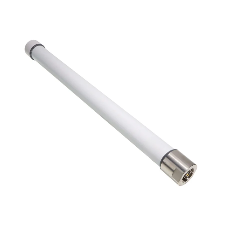
ANTENNA-2000 — Omnidirectional Antenna for use with Access2000 Gateways
Six decibels of omnidirectional gain, which on this post's model is roughly the difference between a 34 m and a 21 m planning radius across an ordinary plant floor. Worth having, and worth understanding: it buys distance, not penetration, so it will not rescue a gateway that is on the wrong side of a wall. Note that two are required per gateway — budget them as a pair, not as an accessory.
- Part number
- ANTENNA-2000
- Gain
- 6 dBi gain improves coverage and signal strength
- Coverage
- 360° omnidirectional from a single mounting location
- Band
- Optimized 2.4 GHz performance
- Return loss
- Better than -10 dB, minimising reflections
- Quantity required
- Two antennas per ACCESS2000 gateway
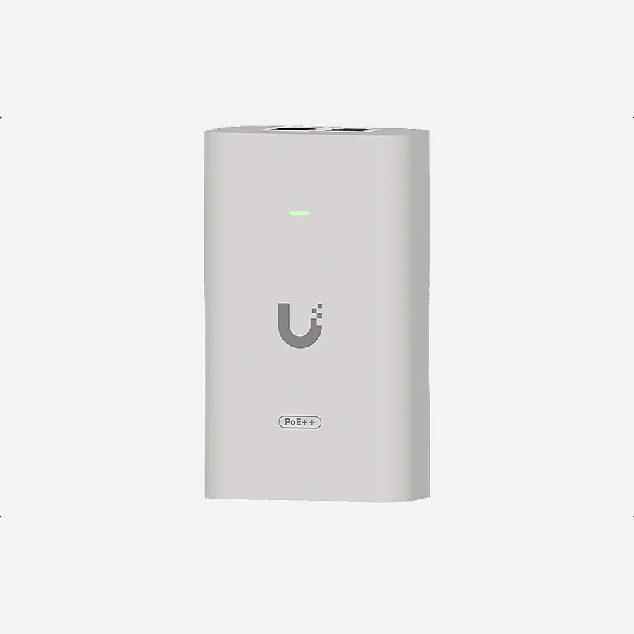
WS-POE — PoE Injector Compatible with CTC Connect Gateways
The part that lets the gateway go where the radio needs it rather than where the socket is — which, on the evidence of this post, is the single most common fixable coverage mistake. An ordinary Ethernet run plus this injector puts both power and data at a mounting position high above the machines, instead of putting the gateway in the switchroom because that is where the power was.
- Part number
- WS-POE
- Description
- PoE Injector Compatible with CTC Connect Gateways
- Rating
- 60 W PoE++ adapter
- Connections
- RJ45 data input, AC cable with earth ground, and PoE++ output
- Protection
- Surge, peak pulse, and overcurrent protection
- Indication
- LED indicator light for status monitoring
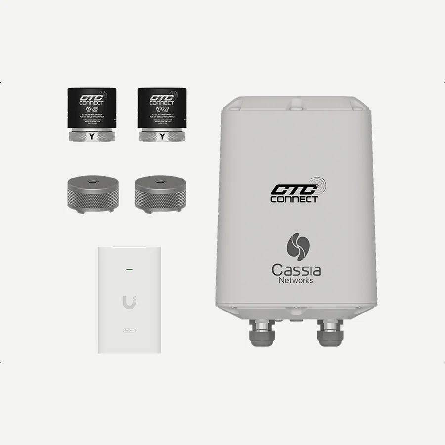
KWSXX-2000 Series — Connect Line Wireless Starter Kit with Access2000 Gateway
The honest first purchase for a plant that has not answered the coverage question yet. A gateway, a choice of two sensors and the mounting hardware is exactly what a survey needs: enough to walk your candidate gateway positions, read the real received level at your real measurement points, and size the rollout from measurements instead of from a model like the one on this page.
- Part number
- KWSXX-2000
- Description
- Connect Line Wireless Hardware Starter Kit with ACCESS2000-POE Long-Range Gateway
- Includes
- A choice of two ConnectSens™ wireless sensors, the ACCESS2000-POE long-range gateway with preinstalled ConnectView™ web app, and essential mounting accessories
From the TIERA store
The kit for this job
What we would actually put in front of someone doing the measurement this post describes — not the whole catalogue.
- Access2000 Series - Long-Range Wireless Gateway & Network ControllerThe ACCESS2000 Series is a long-range wireless gateway and network controller used for connecting CTC Connect compatible products to the data analysis software of your choice via Wi-Fi or Ethernet.Request priceView →
- AntennasBoost your ACCESS2000 Long-Range Wireless Gateway performance with ANTENNA-2000. The antenna offers 360° omnidirectional coverage for consistent wireless coverage in all directions from a single mounting location and optimized 2.4 GHz performance for reliable connectivity for industrial wireless applications.Request priceView →
- PoE InjectorsThe WS-POE is a 60 W PoE++ adapter designed for use with CTC Connect Wireless Gateways. The device contains RJ45 data input, AC cable with earth ground, and PoE++ output. It also offers surge, peak pulse, and overcurrent protection and features a convenient LED indicator light for status monitoring.Request priceView →
- Kwsxx-2000 Wireless Starter Kit with Access2000 GatewayGet started with wireless vibration monitoring using CTC’s KWSXX-2000 Series Connect Line Wireless Starter Kit, your all-in-one solution for remote condition monitoring.Request priceView →
Use cases
Where this shows up in the field
Send us your plant layout and we will do this arithmetic on it before you buy any gateways
TIERA supplies and supports the CTC Connect wireless range in India — the gateways, the omnidirectional antennas, the PoE injectors and the starter kits — and supports them here rather than pointing you at a portal. What is more useful than a quotation is the coverage plan, because the number of gateways is the part of a wireless programme that drives the network runs, the power runs and the lead time.
Send us a layout with your measurement points marked and we will come back with candidate gateway positions, a planning radius for each at an exponent we will justify to you, which points fall inside which circle, where the overlaps and the seams are, and which points the model says will not hold a link at all. Then we will walk it with a real gateway and a real sensor and give you the measured received level at each point, because everything before that sentence is a planning model and we will say so every time.
- Access2000 long-range gateways, with the published ≥ 140 m connected-sensor range and −75 dBm supported floor to plan against
- ANTENNA-2000 omnidirectional antennas, supplied as the pair each gateway requires
- WS-POE injectors, so the gateway position follows the radio rather than the nearest socket
- A written coverage plan per area — candidate positions, planning radius, points in and points out — followed by a walked survey that replaces it
Where this sits on the TIERA learning ladder.
The theory behind this article is covered free, in full, by the TIERA 101 primers: Accelerometer & DAQ Selection 101, AI Condition Monitoring 101. They are self-paced, interactive, and end in an exam and a certificate.
The free primers cover sensor and DAQ selection and what a condition-monitoring data pipeline needs from the measurements feeding it. TCAT adds examined depth: designing a monitoring architecture whose coverage, cadence and record length are derived from the faults being watched for rather than from a supplier's default, and defending that architecture — including the gateway count nobody wants to pay for — in front of the people who sign for it.
TIERA 101 is a free introductory primer, not an accredited ISO certification, and its hours do not count towards the formal training ISO 18436 requires.