Overall or Waveform? What Your Wireless Sensor Can Actually Tell You
The most important spec on a wireless vibration sensor is not range or battery life — it is whether the sensor sends you a waveform or just a number. An overall-only sensor tells you that something changed; a dynamic sensor tells you what. This post does the arithmetic on why, and its simulator grows a synthetic bearing fault over 90 days so you can watch the envelope spectrum name the defect seven weeks before the overall trend crosses its alarm.
Two sensors on the same magnet, answering different questions
Wireless vibration sensors come in two fundamentally different kinds, and the datasheets do not shout about the difference. An overall-level sensor wakes, samples for a moment, computes a handful of scalar values — Peak, RMS, Peak-to-Peak — and transmits those numbers. The waveform they were computed from is discarded inside the sensor; it never crosses the radio. A dynamic sensor transmits the actual sampled waveform, and everything an analyst can do — FFT, envelope analysis, harmonic pattern reading — remains possible downstream.
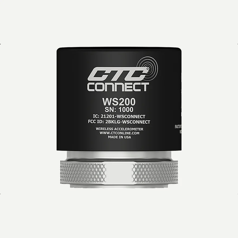
On CTC's Connect line, which TIERA distributes in India, the split is explicit. CTC's WS100 is a triaxial overall sensor: its published datasheet states the output is overall vibration in Peak, RMS and Peak-to-Peak, from a 500 ms reading on a factory-set interval — deliberately, as a process-control and screening instrument. The WS200 (single-axis) and WS300 (triaxial) are dynamic sensors: CTC's family pages state user-programmable sampling up to 25.6 kHz, waveform capture on a schedule or on demand, and the gateway computes FFTs and trends from them. (The WS200/WS300 detailed specification tables — g-ranges, band edges, ingress rating — are available from TIERA on request; we quote here only what CTC publishes openly.)
The two kinds are not a good/better ladder. They are different instruments for different questions, and the honest decision rule — which this post builds — depends on one piece of arithmetic about what an overall number can and cannot contain.
The arithmetic of an overall: energy sums, evidence doesn't
An RMS overall is the square root of the total vibration energy in the measurement band. Energies add in quadrature — and that single fact is the whole story. Suppose a pump runs at 4.0 mm/s RMS, almost all of it the usual 1× and vane-pass content, and an early bearing defect adds 0.5 mm/s of impact energy. The new overall is √(4.0² + 0.5²) = 4.03 mm/s. The defect — clearly present, mechanically real, growing — moved the trended number by 0.68 percent, well inside day-to-day operating scatter from load and temperature. No alarm threshold survives contact with that: set it tight enough to catch 0.68% and it false-alarms on every load swing; set it loose enough to be quiet and the defect walks past it for months.
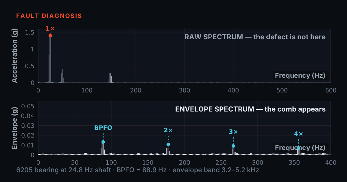
The defect is invisible in the overall not because the sensor is bad but because the overall is a sum, and a small number added in quadrature to a big number disappears. The same defect is unmistakable in the right distribution of that energy: the impacts repeat at the bearing's defect frequency, and an envelope spectrum — the demodulation chain explained at /blog/bearing-envelope-explained and driveable at /blog/envelope-demodulation-simulator — shows a comb of lines at exactly that rate while the overall has not yet moved a full percent. Naming the frequency names the component: outer race, inner race, rolling element, cage. That is the difference between something changed and strip the drive-end bearing, order the part now.
Eventually, of course, the overall does move — late-stage bearing damage raises broadband energy as the spall widens and smears. The overall is not blind; it is late. How late is exactly what the simulator below measures.
Where overall sensors genuinely earn their keep
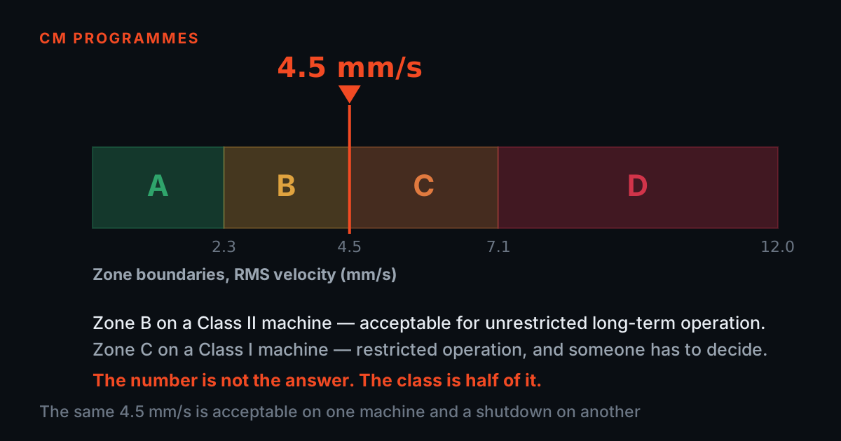
Having shown what overalls miss, honesty requires the other half: an overall-level wireless sensor, used for what it is, is an excellent instrument — and often the correct purchase. Trending is a legitimate and venerable discipline. ISO 20816 severity assessment is itself built on a broadband velocity value in the 10–1,000 Hz band — and it is worth noticing that CTC's WS100 datasheet lists a factory-configured velocity output on a 10 Hz–1 kHz band, which maps directly onto that convention. A fleet of overall sensors reading a few times a day gives every balance-of-plant machine a severity trend it never had, catches the faults that do move the overall early — unbalance growth, misalignment after a coupling job, looseness, late-stage bearing damage — and does it at the lowest cost per point of any permanent instrument. Try your own numbers against ISO zones at /blog/iso-20816-severity-checker.
The failure mode is not the sensor; it is the mismatch. An overall sensor on a machine whose credible failure mode is rolling-element bearing damage, where the maintenance decision is an expensive evidence-based teardown, is a mismatch: when the trend finally fires you still do not know which component, and the P-F runway the wireless cadence bought you has largely been spent. The decision rule that falls out: overalls for machines where the response to an alarm is 'go look' — dynamic sensors for machines where the response needs to be 'replace this specific part'. That is TIERA's framing, but CTC's own product split says the same thing structurally: the WS100 is positioned for process monitoring and screening, the WS200/WS300 for analysis.
Watch 90 days of bearing damage through both windows
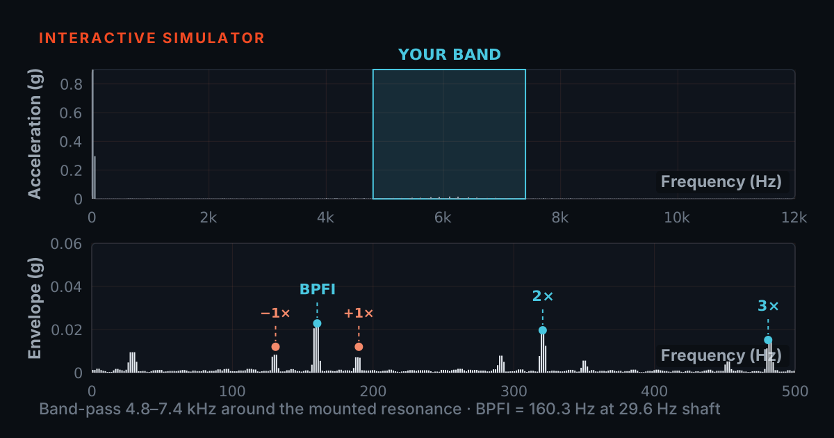
The simulator below grows a synthetic outer-race bearing fault on a 1,440 RPM pump over 90 days and shows every day through both windows at once. The signal is honest DSP, computed live in your browser, and — to be completely clear — it is a simulation, a model of a typical progression, not data from any real machine. Each day's signal is 1,024 samples at 8,192 S/s: a 24 Hz shaft component, a 168 Hz vane-pass component from seven vanes, broadband noise, and a train of decaying 2.8 kHz resonance bursts repeating at 88 Hz — the outer-race rate. Severity grows quadratically; in the late stage the broadband floor rises too, as a widening spall stops producing crisp impacts and starts producing rough running — that floor rise is what eventually moves the RMS.
The top panel is what an overall-only sensor would radio out: one RMS number per day, trended against an alarm line you control. The bottom panels are what a dynamic sensor enables: the day's waveform, and its envelope spectrum computed by the same band-pass + Hilbert chain as our envelope simulator, with a lock lamp measuring how far the 88 Hz comb stands above the floor. Both views are computed from the same signal — the only difference is how much of it survives the radio.
Synthetic 1,440 RPM pump (24 Hz shaft, 168 Hz vane pass), seeded outer-race fault, BPFO = 88 Hz, housing resonance 2.8 kHz. Envelope band fixed at 2.3–3.3 kHz. 1,024 samples at 8,192 S/s per day, computed live. A simulation of a typical progression — not a real machine.
—
What the dynamic sensor changes downstream
A waveform over the radio changes more than early warning. It changes what kind of conversation your team can have. With CTC's dynamic sensors, the gateway computes FFTs and trends alongside the raw waveform, readings can be triggered on demand — an analyst who sees something odd can ask for a fresh capture now rather than waiting for the schedule — and the reading configuration (sampling frequency, record length, interval) is user-programmable per sensor, so a gearbox point and a pump point need not share settings. CTC's MQTT manual documents record lengths from 1,600 to 25,600 samples per reading, with the actual sampling rate and Fmax reported in each payload — which means your own software, or TIERA's TVIB, can consume the raw data without a proprietary lock-in.
Be equally clear-eyed about what it does not change. CTC's own brochure describes the bundled ConnectView software as basic vibration tools, designed to integrate with third-party analysis software rather than replace it — a piece of vendor honesty worth rewarding. The waveform gives you the possibility of diagnosis; the diagnosis still needs an analyst, or analysis software, or both. A dynamic sensor fleet with nobody reading the spectra is an expensive overall sensor fleet. Budget the analysis capability — training, software, or a service contract — with the same seriousness as the hardware, or buy overalls and be honest about it.
One more asymmetry worth naming: you can always compute an overall from a waveform — the simulator above does it live — but no amount of software recovers a waveform from an overall. The scalar sensor made that decision inside its case and it is permanent. When in doubt between the two classes on a machine that matters, the waveform keeps your options open; the overall forecloses them.
The decision rule, and the verification step nobody should skip
The allocation that falls out of all this, stated as TIERA's engineering judgement: overall-level sensors for balance-of-plant machines where trending is the goal and an alarm's response is an investigation — with a velocity-band configuration that maps onto ISO 20816 severity zones where available. Dynamic sensors for machines whose teardown decisions must be justified by evidence — anything with expensive bearings, gearboxes, or a spares lead time measured in weeks. Wired instrumentation where the physics gates in the companion guide at /blog/wired-vs-wireless-vibration-monitoring rule wireless out entirely.
And whichever class raises the flag: verify before you strip. A wireless alarm — scalar or spectral — is a screen, not a verdict. The professional close-out is a wired measurement with a portable analyser at the flagged point: full bandwidth, an analyst's band placement (practise it at /blog/envelope-demodulation-simulator), a proper mount (see /blog/mounting-wireless-vibration-sensors for why the mount decides what the sensor can see), and a decision you can sign. The wireless fleet's job was to tell you where to point that effort — and used this way, it does that job supremely well.
TIERA instruments that do this work.
CTC WS200 Series ConnectSens Wireless Sensor
The dynamic-waveform class this post argues for on machines that matter: real time waveforms on a schedule or on demand, user-programmable per point.
- Type
- Single-axis dynamic vibration + temperature
- Radio
- Bluetooth Low Energy 5.2, 1,200 ft (366 m) line-of-sight
- Readings
- Scheduled or on-demand; user-programmable via ConnectView
- Battery
- User-replaceable, up to 4 years (CTC, at 2 readings/day)
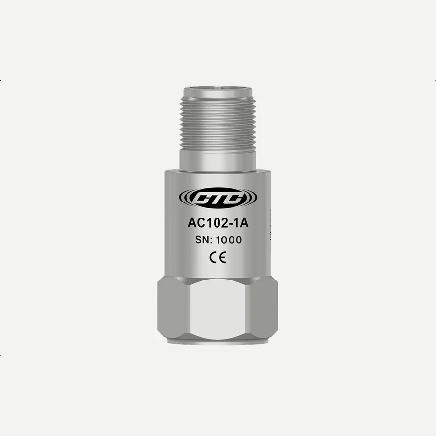
CTC 100 mV/g Standard Size Accelerometers
The wired verification measurement every wireless alarm deserves before money is spent on a teardown.
- Sensitivity
- 100 mV/g
- Dynamic range
- ±80 g
- Family
- AC102 / AC104 / AC150 and variants

PhonoVibe Q — 4-Channel IEPE DAQ
The portable analysis chain that turns a wireless flag into a signed diagnosis — full-bandwidth capture and TVIB's envelope tools.
- Channels
- 4, simultaneous, 24-bit
- Bandwidth
- 0.5 Hz – 60 kHz at 128 kHz sampling
- Software
- TVIB TSAP201 included
From the TIERA store
The kit for this job
What we would actually put in front of someone doing the measurement this post describes — not the whole catalogue.
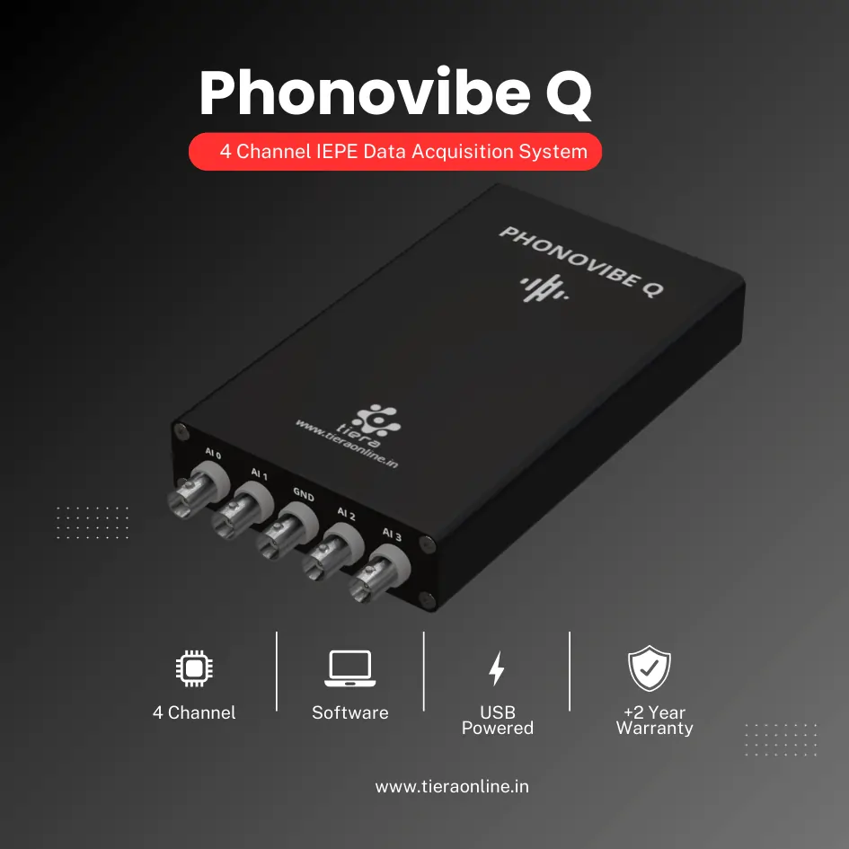 4 Channel IEPE Data Acquisition System – Phonovibe QFour Channels Standard plug & play USB Powered Take data from accelerometers, microphones, hammers, or any other IEPE Sensors T- VIB Software to acquire time waveforms, frequency spectra, overall vibration levels, FRF’s and octave measurements ** Windows 10 or above Operating System ** T-VIB Software base version comes with Time and Spectrum with Post processor TSAP 201. Check out TVIB Software regarding more module options.₹2,88,000View →
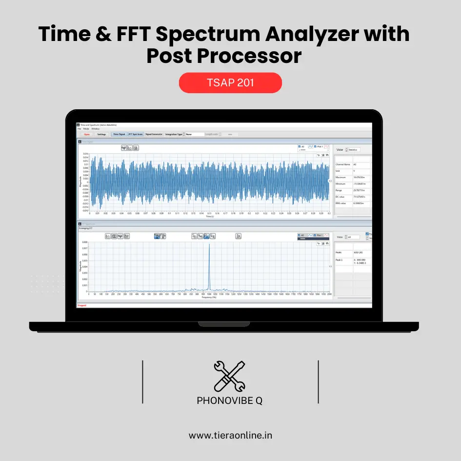 TSAP 201 -Time & FFT Spectrum Analyzer with Post Processor (Phonovibe Q)Use Cases Bump Test Product Development Off route Machine Vibration analysis. Drop Test Product Development & Research₹34,560View →
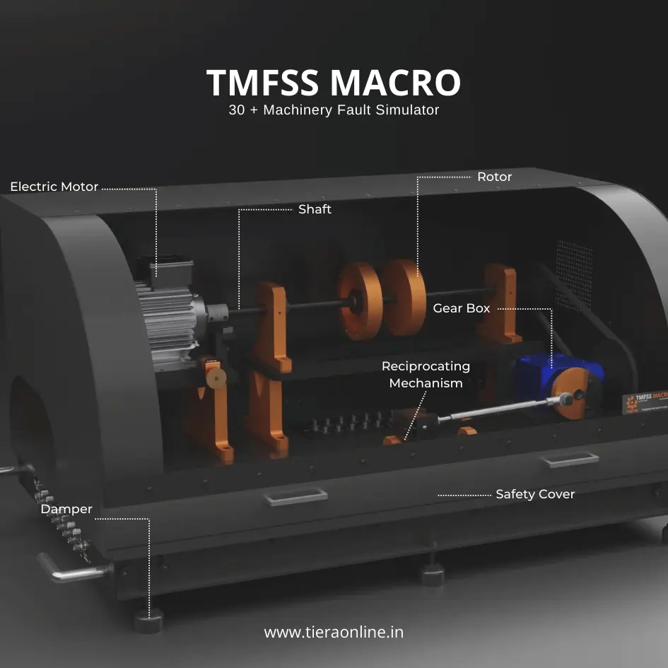 Machinery Fault Signature SimulatorTiera’s Machine Fault Simulator (TMFSS) is a valuable tool for industries and researchers, simulating over 30 real-world faults such as: Bearing faults: outer race defects, inner race defects, cage defects. Motor faults: stator faults, rotor faults, electrical unbalance. Gearbox faults: gear wear, misalignment, gear tooth damage. Etc..₹13,53,600View →
Use cases
Where this shows up in the field
Match the sensor class to the decision it must support — we will help you split the fleet
TIERA supplies the full CTC Connect wireless family in India — overall-class and dynamic-class sensors, the ACCESS360 gateway and mounting hardware — alongside the wired accelerometers and the PhonoVibe analysis chain that closes the loop on every alarm. Detailed specification tables for the WS200 and WS300 dynamic sensors are available on request.
Send us your machine list and we will mark, machine by machine, which class each point justifies — and where an overall sensor is honestly all you need, that is what we will quote.
- CTC dynamic wireless sensors for evidence-based teardown decisions
- CTC overall wireless sensors for balance-of-plant trending
- PhonoVibe + TVIB for the wired verification measurement
- Analyst training so the waveforms you pay for actually get read
Where this sits on the TIERA learning ladder.
The theory behind this article is covered free, in full, by the TIERA 101 primers: Bearing & Gear Analysis 101, Machinery Fault Diagnosis 101. They are self-paced, interactive, and end in an exam and a certificate.
The free primers teach the envelope chain this post's simulator runs; TCAT Cat II adds the discipline of reading real spectra and defending a teardown call — the skill that makes a dynamic sensor fleet worth its price.
TIERA 101 is a free introductory primer, not an accredited ISO certification, and its hours do not count towards the formal training ISO 18436 requires.