Tune the Band, Find the Bearing: An Interactive Envelope Demodulation Simulator
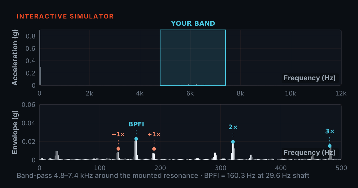
Envelope analysis is a tuning job: park a band-pass window on the bearing's ring frequency and the defect comb appears; slide it off and the comb dies. This simulator computes the whole chain live — synthesised impacts, a real band-pass filter, a real envelope spectrum — so you can feel it, like tuning a radio.
The quiet station at the top of the dial
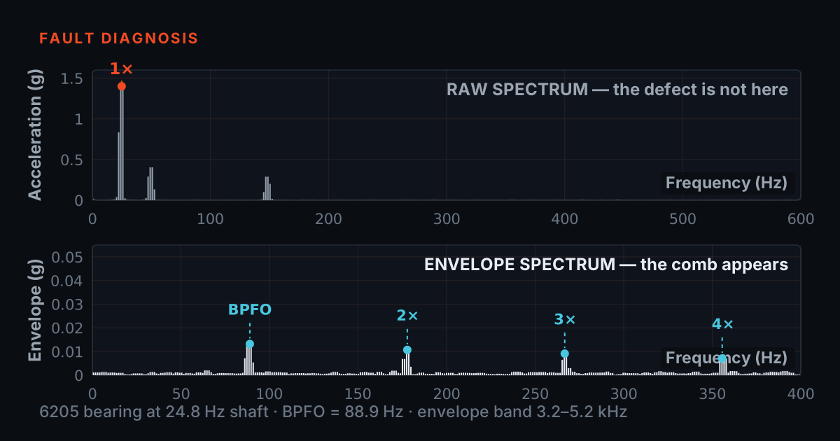
Tune an old radio at night and the dial is crowded at one end: powerful local stations blasting over each other, easy to find, telling you nothing new. The station you actually want is far up the dial — faint, but alone, with no neighbour to drown it. Finding it is not about volume. It is about putting the window in the right place. Envelope analysis is exactly this. The loud stations are the machine's steady components: 1x running speed, blade pass, gear mesh. The faint lonely station is the bearing housing's structural resonance, up in the kilohertz range, which rings briefly every time a rolling element strikes a defect.
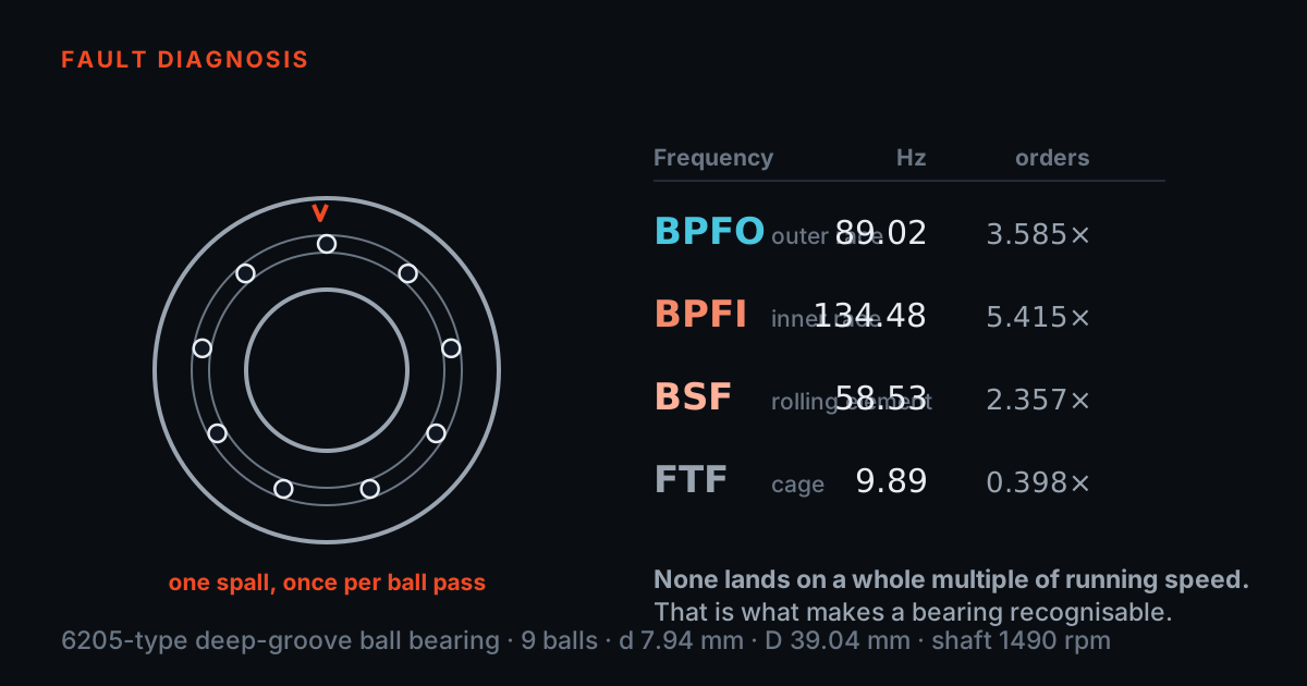
In the companion explainer at /blog/bearing-envelope-explained we walked through why that works: why the raw spectrum hides an early defect, what BPFO, BPFI, BSF and FTF mean, and what the demodulation chain does step by step. This post is the other half of the lesson — the part reading cannot give you. Below is a live simulator that computes the full chain on every slider move. Your job is to tune the band-pass window until the defect comb locks in. Miss the resonance and the comb is simply not there.
What this simulator actually computes
- The number to hunt for is 88 Hz — the outer-race rate (BPFO) for this bearing at 1,500 RPM — and its harmonics at 176 and 264 Hz.
- The impacts ring at 2.5 kHz with a time constant of about 1.5 ms. That ring, not the impact energy itself, is what the band-pass window has to sit on.
- Nothing is canned: the band-pass is an ideal frequency-domain filter, the envelope is the magnitude of the analytic signal, and the comb appears because the mathematics put it there.
Nothing below is a canned animation. On every slider move the simulator synthesises 1,024 samples at 8,192 samples per second — an eighth of a second of signal. Into it go a 25 Hz shaft component (1,500 RPM), a 150 Hz blade-pass component from a six-blade fan, broadband Gaussian noise, and the fault: a train of micro-impacts repeating 88 times a second, the outer-race rate (BPFO) for this bearing at this speed. Each impact is a short decaying burst of 2.5 kHz ringing with a time constant of about 1.5 ms — the housing resonance being struck and dying away.
The processing is the real chain, computed live. Your band-pass window is applied as an ideal filter in the frequency domain: FFT the signal, keep only the bins inside the window, discard the rest. The envelope is the magnitude of the analytic signal — the textbook Hilbert-transform route, computed by the same FFT. That envelope is windowed and FFT'd again to give the envelope spectrum. So when a comb appears at 88 Hz and its harmonics, it is there because the mathematics put it there: the spacing equals the impact rate you dialled in, and no line in the plot was drawn by hand.
Tune the band, find the bearing
The window starts in the wrong place — parked at 900 Hz, where there is nothing but the skirts of the machine's steady components and a slice of noise floor. The top strip is your dial: the live raw spectrum with the band window drawn on it. When defect severity is above zero, look for the modest hump the impacts raise around 2.5 kHz. That hump is the station you are hunting.
Drag the band centre up the dial and watch all three panels react. In the band-passed panel, the moment the window covers the resonance, the shapeless residue snaps into a train of sharp repeating bursts, and the orange envelope traces their outline. In the envelope spectrum, a comb rises at 88 Hz, 176 Hz, 264 Hz — the lock lamp reports how far the comb stands above the floor. Slide the window off again and the comb collapses, even though the defect never changed. That is the whole discipline of envelope analysis in one gesture: the fault is only visible from where the machine is quiet.
Machine: 1,500 RPM (25 Hz shaft), six-blade fan (blade pass 150 Hz). Seeded fault: outer race, BPFO = 88 Hz. Housing resonance near 2.5 kHz. Record: 1,024 samples at 8,192 S/s, computed live.
Why sliding off the band kills the comb
- Everything follows from one ratio: signal inside the band versus everything else inside the band. Park the band wrong and both halves move against you at once.
- The envelope of a clean bump train FFTs into a comb at the repetition rate. The envelope of noise FFTs into a floor — which is what an off-band measurement is actually showing you.
The comb lives or dies by what the filter lets through. Each impact is tiny in total energy, but that energy is concentrated around the resonance, where the rest of the machine is silent — so inside a well-placed band the impacts are the loudest thing there, and the envelope faithfully traces one bump per impact. An FFT of a clean bump train is a comb at the repetition rate. Everything follows from that one ratio: signal inside the band versus everything else inside the band.
Park the band at 900 Hz instead and both halves of the ratio move against you. Most of the impact's ringing energy is outside the window, so the bursts barely register; meanwhile the skirts of blade pass, its harmonics, and plain broadband noise are inside it. The envelope now traces noise, and the FFT of noise is a floor, not a comb. The defect did not get better — you just tuned to a station where it does not broadcast. That is also why 'no comb' on a real machine is only meaningful if you know the band was in the right place first.
How wide should the window be?
- Too narrow clips the burst's own bandwidth: each impact smears into a long ripple and the comb's higher harmonics — often the most convincing part of the pattern — fade first.
- Too wide readmits blade-pass harmonics, mesh energy and a broad slice of noise floor, which raises the floor under the comb.
- The working rule is to cover the resonance hump generously while staying clear of the strong deterministic components below it.
Centre frequency gets you to the right neighbourhood; width decides what you keep once you are there. Too narrow and you clip the burst's own bandwidth: a short impact needs a spread of frequencies to look short, and a very narrow filter smears each burst into a long ripple. The envelope loses its crisp one-bump-per-impact shape, and the higher harmonics of the comb — often the most convincing part of the pattern — fade first. In the simulator, pinch the width down to 100-200 Hz on the resonance and watch exactly that happen.
Too wide and you readmit what you worked to exclude: harmonics of blade pass, mesh energy, and a broad slice of noise floor ride into the envelope and raise the floor under the comb. The practical rule is to cover the resonance hump generously — comfortably wider than several multiples of the highest fault frequency of interest — while staying clear of the strong deterministic components below. On real machines analysts often confirm the choice empirically, exactly as you are doing here: nudge the band, and trust the setting that makes the comb stand tallest above its floor.
A representative case — and where to practise the tuning
A representative case, not a specific customer: an analyst inherits a monitoring point on a fan drive-end where enveloping has 'never shown anything'. The stored setup reveals why — the demodulation band was left at a default a long way below the housing resonance, close to where this simulator starts. Re-measuring with the band moved onto the hump visible in a high-frequency spectrum, a clean comb appears at the outer-race rate, small but unambiguous, weeks of margin still in hand. Nothing about the machine changed between the two readings; only the window did. It is the off-band trap from the panels above, played out on a real setup screen.
The instinct for where to put the band is trainable, and fastest to train on faults you can trust. A TMFSS simulator with seeded bearing defects — outer race, inner race, cage, rolling element — lets you tune a real band on a real signal and check the comb against a rate you know is true, exactly as you just did on the canvas. For the theory underneath, the free Bearing & Gear Analysis 101 primer at 101.tieraonline.in covers it step by step — it is a free primer, not an accredited ISO certification. When you want the formal credential, TIERA's TCAT programme runs Cat I through Cat IV analyst training (see /services), with proctored examinations at exams.tieraonline.in.
TIERA instruments that do this work.

PhonoVibe Series — Sound & Vibration DAQ
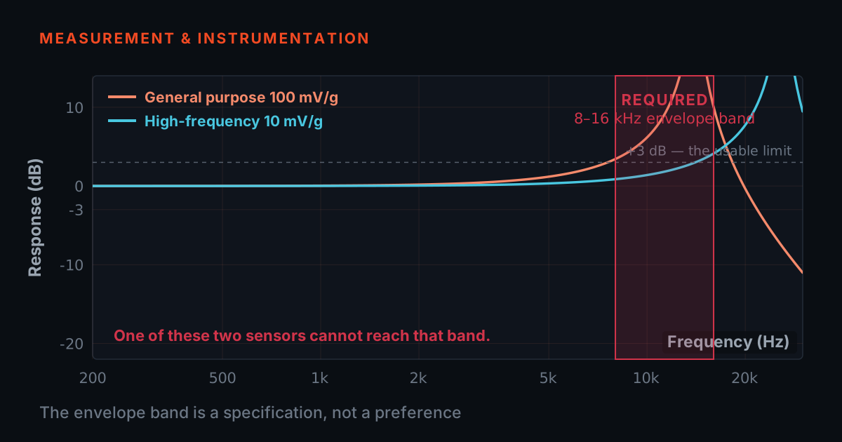
The whole technique depends on reaching the resonance band — Q/O/HD sample at 128 kHz over 0.5 Hz – 60 kHz, so real housing resonances sit inside the measured range.
- Bandwidth (Q/O/HD)
- 0.5 Hz – 60 kHz at 128 kHz sampling
- ADC resolution
- 24-bit, simultaneous sampling
- Channels
- 2, 4, 8 or 16 (BNC)
- Sensor power
- 24 V, 4 mA (IEPE/ICP/CCLD)
- TEDS
- Supported

TVIB — Sound & Vibration Analysis Software
The band-tuning you did by slider, done for real: FIR/IIR band-pass filtering, then harmonic and sideband cursors to lay a ruler over the comb — with recorded signals re-processable on a different band later.
- Filtering
- FIR and IIR filters
- FFT size
- Up to 102,400 points
- Cursors
- Harmonic, band and sideband, in time and frequency
- Post-processing
- Signal recording and re-processing
- Base module
- TSAP201 — free with every PhonoVibe
Sensors & Accessories
The high frequencies you are tuning to are the first thing a loose fixture throws away — rigid mounts and low-noise cabling keep the resonance band alive from sensor tip to DAQ input.
- Accelerometer
- TACPB-10T3 uniaxial MEMS IEPE
- Permanent mount
- TMB-101-1-A SS304 triaxial block
- Route mount
- TMA-101-1 magnetic mount
- Cabling
- CA-101 low-noise coaxial, 5 m, 10-32 to BNC
From the TIERA store
The kit for this job
What we would actually put in front of someone doing the measurement this post describes — not the whole catalogue.
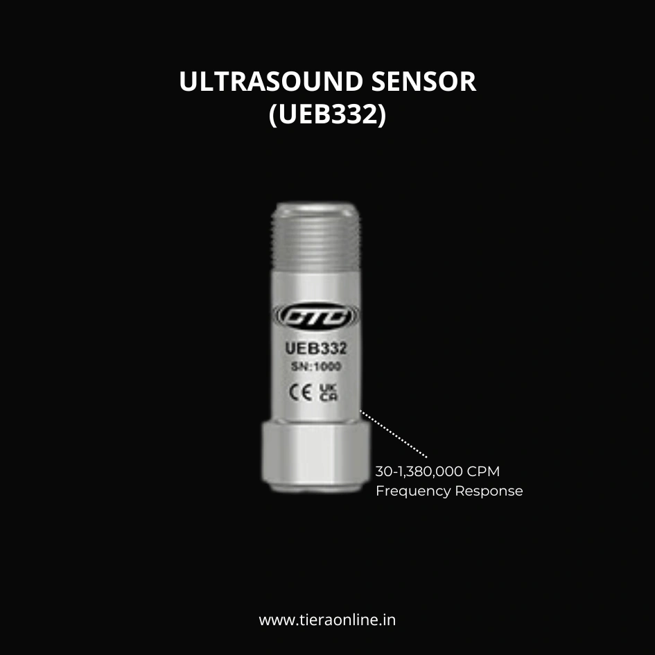 UEB332, ULTRASOUND SENSORCTC’s High Frequency Ultrasound Accelerometer. High Amplitude Resonance Peak for Stress Wave Measurement Techniques. It works on the IEPE Amplifier Technology.₹44,560View →
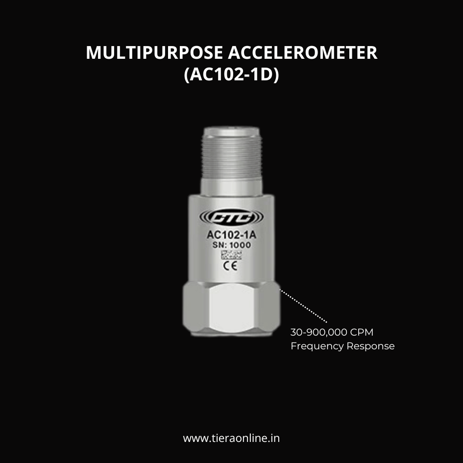 AC102-1D, MULTIPURPOSE ACCELEROMETERMULTIPURPOSE ACCELEROMETER, TOP EXIT 2 PIN CONNECTOR, 100 MV/G, ±10% 30-900,000 CPM Frequency Response (±3dB) -58 to 250 °F (-50 to 121 °C) Temperature Range Welded, Hermetic Sealing CTC’s Best Selling, Multi-Purpose Sensor Ideally Suited for Thousands of Applications₹14,750View →
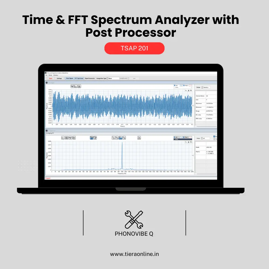 TSAP 201 -Time & FFT Spectrum Analyzer with Post Processor (Phonovibe Q)Use Cases Bump Test Product Development Off route Machine Vibration analysis. Drop Test Product Development & Research₹34,560View →
Use cases
Where this shows up in the field
The real version of this dial: hardware that reaches the band, software that tunes it
The simulator's whole lesson depends on being able to reach and resolve the resonance band — and that is a hardware property before it is a technique. PhonoVibe Q, O, and HD sample at 128 kHz with 24-bit resolution across a 0.5 Hz – 60 kHz bandwidth, with IEPE sensor power built in, so real housing resonances sit comfortably inside the measured range. The band-tuning you did by slider, TVIB's TSAP201 does for real: FIR and IIR band-pass filtering, FFT up to 102,400 points, and harmonic, band, and sideband cursors to lay a ruler over the comb — with recorded signals re-processable later if you want to try a different band.
None of it survives a bad mounting: the high frequencies you are tuning to are the first thing a loose fixture throws away, which is why the accessory range runs from SS304 triaxial mounting blocks and adhesive pads for permanent points to magnetic mounts for routes, with low-noise coaxial cabling to keep triboelectric hash out of a small signal. And if you want to build the tuning instinct on faults you can trust, a TMFSS simulator with seeded outer-race, inner-race, cage, and rolling-element defects gives you a comb whose true rate you already know.
- PhonoVibe Q / O / HD — 24-bit, 128 kHz sampling, 0.5 Hz – 60 kHz bandwidth, IEPE power: reaches the resonance band this post is about
- TVIB TSAP201 — FIR/IIR band-pass, FFT to 102,400 points, harmonic and sideband cursors, signal recording and re-processing
- Mounting and cabling — SS304 triaxial blocks, magnetic mounts, low-noise coaxial cables to preserve the high-frequency path
- TMFSS — seeded bearing defects (outer race, inner race, cage, rolling element) to practise band placement against a known truth
Where this sits on the TIERA learning ladder.
The theory behind this article is covered free, in full, by the TIERA 101 primers: Bearing & Gear Analysis 101. They are self-paced, interactive, and end in an exam and a certificate.
The free 101 primers at 101.tieraonline.in teach the theory behind this simulator; TCAT Cat I-IV adds structured analyst training with proctored examinations at exams.tieraonline.in — the credential that says you can do this on a real machine.
TIERA 101 is a free introductory primer, not an accredited ISO certification, and its hours do not count towards the formal training ISO 18436 requires.