Choosing an Industrial Accelerometer: Three Numbers That Fight Each Other
Sensitivity, dynamic range and noise floor are not three specifications to compare in a table — they are one decision, and improving any of them costs you another. A selection guide with a live bench that computes the clip level, the noise floor and the usable band, and refuses to price a measurement your mount cannot deliver.
Three numbers decide it, and they fight each other
- Sensitivity, clip level and reachable bandwidth all come out of the same lump of metal and ceramic, which is why no sensor is best at all three.
- Dynamic range — the distance in decibels between the clip level and the noise floor — is the only figure that says what the sensor can actually do.
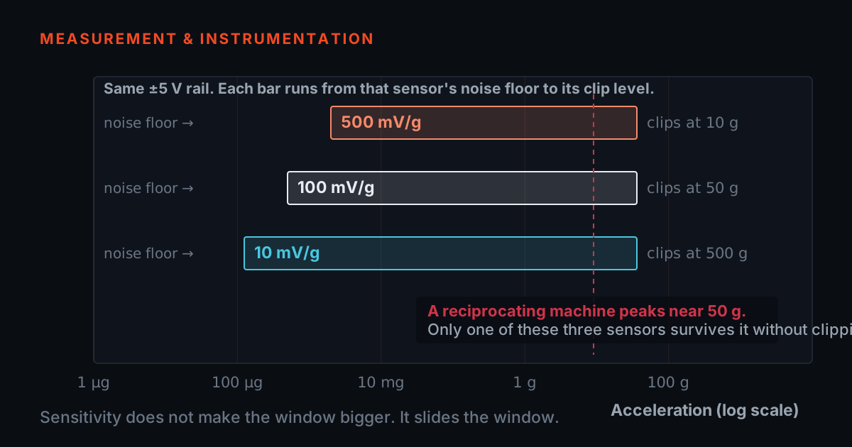
- Push sensitivity up and the clip level comes down by exactly the same factor. There is no setting where all three improve.
Open any accelerometer datasheet and you get a table: sensitivity in millivolts per g, a frequency response in hertz, a measurement range in g, a spectral noise density in micro-g per root hertz, a mounted resonance, a temperature range, a weight. Most buyers read that table as a list of independent qualities and reach for the sensor that looks best on the line they care about — usually sensitivity, because a bigger number sounds like a better sensor. It is the wrong reading, and it is the reason a lot of otherwise sensible condition-monitoring programmes are built on the wrong hardware.
Three of those lines are not independent at all. They are three views of the same physical object, and they are locked together. Sensitivity sets how many millivolts you get per g of acceleration. The output has a fixed voltage swing to play with, so sensitivity also sets the largest acceleration you can measure before the output flattens against that limit — the clip level. The noise floor sets the smallest acceleration you can distinguish from the sensor's own hiss. The distance between those two, in decibels, is your dynamic range, and it is the only figure that says what the sensor can actually do. Push sensitivity up and the clip level comes down by exactly the same factor. There is no setting where all three improve.
Underneath the table there is one mechanism, and it explains the whole trade. A piezoelectric accelerometer is a seismic mass pressed against a piezoelectric crystal. Acceleration of the base makes the mass push on the crystal; the crystal produces charge in proportion; a built-in amplifier turns that charge into a voltage on the same two wires that power it. A bigger mass produces more charge for the same acceleration — more sensitivity — but a bigger mass on the same crystal stiffness also lowers the resonance of the assembly, which lowers the frequency the sensor can reach. Sensitivity, range and bandwidth all come out of the same lump of metal and ceramic. That is why they trade.
Sensitivity is not quality
The single most common selection error is treating a higher sensitivity as a better sensor. It is not a quality figure. It is a scaling factor, and the scale it sets runs in both directions. A 500 mV/g sensor gives you five times the volts per g of a 100 mV/g sensor — and reaches its output limit at exactly one fifth of the acceleration. The trade is not approximately linear or usually linear. It is exactly linear, because it is the same division done twice.
Work it through with real arithmetic. Take an industrial IEPE sensor whose amplifier can swing about five volts either side of its bias point before it stops. At 100 mV/g, five volts is fifty g: the sensor reports honestly up to fifty g peak. At 500 mV/g, the same five volts is ten g. Put that 500 mV/g sensor on a machine that produces twenty g peaks at the bearing housing — a reciprocating compressor, a hammer mill, a machine with looseness that is already knocking — and the output runs into the limit twice per cycle. It does not fail. It does not warn you. It flattens the tops of the peaks and hands you a waveform that looks a little squared off.
That squared-off waveform is worse than a missing measurement, because it is a measurement that lies in a specific and misleading direction. Flattening a peak is a nonlinearity, and a nonlinearity generates harmonics that were never on the machine. You get a tidy series of harmonics of running speed appearing in the spectrum, which is the classic signature of mechanical looseness, and an analyst who trusts the data diagnoses looseness on a machine that does not have any. The clipping also suppresses the true peak amplitude, so the overall level trends down at the same time. Nobody looking at that spectrum has any reason to suspect the sensor.
The rule that falls out is not 'buy less sensitivity'. It is: pick the sensitivity that fits the machine you are putting it on, and check the arithmetic before you buy. Five hundred millivolts per g is the right answer on a slow agitator, a paper-machine roll or a cooling-tower gearbox, where amplitudes are small and the noise floor is what limits you. It is the wrong answer on anything that impacts.
The rail you never see
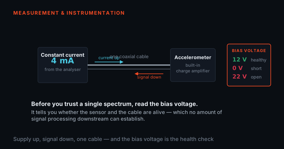
Clipping is arithmetic, not a mystery, and the arithmetic is worth doing explicitly because the number involved appears on almost no datasheet in the form you need it. An IEPE accelerometer is powered by a constant current — typically two to ten milliamps — sent up the signal wire. The sensor's internal amplifier sits at a bias voltage, somewhere in the region of ten to fourteen volts, and the signal rides on top of that bias as a swing about it. The usable swing is bounded below by the amplifier's minimum working voltage and above by the supply voltage of the current source. What is left is the rail: the volts you actually have, either side of bias, before the amplifier saturates.
So the clip level is the rail divided by the sensitivity. Five volts of usable swing at 100 mV/g is fifty g peak. The same five volts at 500 mV/g is ten g. The same five volts at 10 mV/g is five hundred g. Nothing else enters. This is why the measurement-range line on a datasheet — the ±g figure — is not an extra specification but the same statement in different units, and why a sensor whose stated range sits comfortably above your machine's peaks is what you are checking for.
Two practical consequences follow, and both are easy to miss. First, the rail depends on the conditioner, not only on the sensor. A twenty-four volt supply gives an amplifier more room than an eighteen volt one; a long cable with significant resistance eats into it; a conditioner running at the bottom of its compliance range quietly reduces your headroom. If you have ever seen a channel clip in the field on a machine where the bench said it should not, the supply is the first place to look — /blog/iepe-signal-conditioning-explained goes through that end of the chain. Second, the clip level applies to the instantaneous peak, not to the RMS or overall level you trend. A machine whose overall velocity looks unremarkable can still be delivering short high-g impacts at the bearing housing — that is exactly what an early bearing defect does — and it is the impacts that hit the rail. Trending overall levels will never show you that it is happening.
The habit worth building is to work in peak g at the sensor and leave margin. Take the largest peak acceleration you expect at that point, double it for the transients you have not seen yet, and require the clip level to be above that. Then choose the highest sensitivity that still passes, because everything below the clip level is where the resolution argument lives.
The noise floor sets the smallest fault you can see
- Noise integrates as density × √bandwidth: 100 µg/√Hz over a 10 kHz band is 10 mg RMS, and over 100 Hz the same sensor gives 1 mg.
- Narrowing Fmax is the cheapest improvement anywhere in the measurement chain, and it costs exactly one thing — everything above the new limit.
- The lowest-noise sensors tend to be the highest-sensitivity ones, so the noise argument and the clipping argument pull in opposite directions and the machine decides which wins.
At the other end of the range, the limit is the sensor's own noise. It is quoted as a spectral noise density in micro-g per root hertz, usually at a stated frequency such as one kilohertz, and the odd unit is the useful part: it tells you that the noise you actually get depends on how much bandwidth you look through. Broadband noise integrates as the density multiplied by the square root of the bandwidth. That square root is the whole story.
Put numbers on it. A sensor specified at 100 micro-g per root hertz, analysed over a ten kilohertz band, gives a noise floor of 100 micro-g times the square root of ten thousand — that is, times one hundred — which is ten milli-g RMS. Narrow the analysis band to one hundred hertz and the same sensor gives one milli-g. You have improved your smallest detectable signal by a factor of ten and changed nothing but a setting on the analyser. Nothing was bought and nothing was mounted differently.
This is the cheapest improvement available anywhere in the measurement chain, and it costs exactly one thing: Fmax. Narrowing the band means you can no longer see anything above the new upper limit. That is a real cost when the fault you are hunting lives up there — bearing ring frequencies and gear mesh live in the kilohertz — and no cost at all when it does not. A slow agitator at twelve revolutions per minute has nothing above a few tens of hertz worth recording, so analysing it over a ten kilohertz band buys nothing and pays for it by burying the very small signals that a slow machine produces under a hundred times more noise than necessary.
The other lever is the sensor itself. Noise density varies enormously across the market — from a couple of micro-g per root hertz on a quiet industrial unit to several hundred on a cheap one or a very-high-range one — and the sensors with the lowest noise tend to be the ones with the highest sensitivity, because sensitivity is bought with mass and more mass means more signal for the same electronic noise. So the noise argument pushes toward high sensitivity, the clipping argument pushes away from it, and the machine decides which one wins. That is the fight this post is about, and it is the thing the bench below lets you settle in a few seconds instead of a few emails.
The band the sensor can actually reach
- The datasheet resonance is measured stud-mounted on a prepared flat spot face. It is the ceiling of what the sensor could do, not what it will do on your machine.
- The working ceiling is one third of the mounted resonance: a 30 kHz stud gives 10 kHz, a 4.2 kHz magnet gives about 1.4 kHz.
- 1.4 kHz is below where bearing and gear evidence lives — so the mount, not the sensor, usually sets the top of your band.
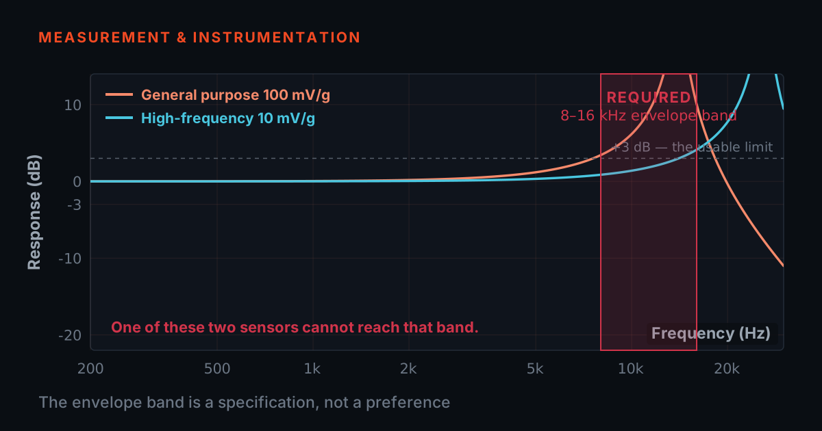
The third number is the one most often taken at face value. A datasheet quotes a frequency response as a range with a tolerance — commonly ±3 dB, sometimes ±10 % or ±5 % for a tighter grade. Read the tolerance, not just the range. Three decibels is not a rounding error: at the upper edge, where the response is already rising toward the sensor's resonance, +3 dB means the sensor reports an amplitude forty-one per cent higher than the machine produced. At the lower edge, −3 dB means twenty-nine per cent lower. Those are the limits of the quoted range, not working points. If you set alarm thresholds from data taken at the edge of a ±3 dB band, you have built a forty-per-cent error into the threshold.
The upper limit exists because of the resonance. The mass-on-a-crystal assembly has a natural frequency, and near it the sensor amplifies. Above it, the sensor stops following the surface and the response collapses. Datasheets quote a resonant frequency — but that figure is measured with the sensor mounted the best way it can be mounted, on a stud, on a prepared flat spot face. It is the ceiling of what the sensor could do, not what it will do on your machine.
What matters in the field is the mounted resonance: the resonance of the sensor as attached, through whatever mount you actually used. The mount is a spring, and a softer spring gives a lower resonance. A stud on a prepared spot face is stiff and lands somewhere near thirty kilohertz for a typical industrial sensor. A good flat magnet on clean, flat, bare metal is far softer and lands near four kilohertz. A handheld probe is softer again. The companion posts at /blog/sensor-mounting-bandwidth-simulator and /blog/magnetic-mount-selection work through those numbers in detail; the point here is only that the mount, not the sensor, usually sets the top of your band.
The working rule TIERA uses — and the same rule those two posts use, deliberately, so that the three articles agree — is one third of the mounted resonance. At a third of the resonance the amplification is about one decibel, which is a small enough error to ignore and small enough not to drift as the mount ages. A thirty-kilohertz stud mount therefore gives a ten-kilohertz working ceiling. A 4.2 kHz magnet gives about 1.4 kHz. That second number is the one that surprises people: a magnet mount that feels immovable in the hand has quietly capped your honest band at 1.4 kHz, which is below where bearing and gear evidence lives.
Drive the trade-off yourself
Everything above is three lines of arithmetic. Here they are as a bench you can drive. Set a sensitivity and a rail and it computes the clip level. Set a noise density and an analysis band and it computes the noise floor over that band, and the dynamic range between the two. Set a mounted resonance and it computes the working ceiling. The presets across the top load the three worked selections from the next section, plus one case that fails.
One behaviour is deliberate and worth watching for. If you ask for an analysis band that sits above the ceiling your mount can deliver, the bench will not print a noise floor or a dynamic range for it. It says so instead, and tells you the largest band that mount can actually support. A number there would be a number for a measurement nobody can make: above the ceiling, the amplitude in the spectrum is the mount ringing rather than the machine moving, and computing a tidy noise floor across it would dress that up as a specification. Load the 'magnet on a painted pipe' preset and you will see it refuse.
- Clip level
- —
- Noise floor over the band
- —
- Usable ceiling (fn/3)
- —
- Dynamic range
- —
This is a simulator. Clip level is the rail divided by the sensitivity; the noise floor is the density times the square root of the analysis band; the usable ceiling is one third of the mounted resonance, the same rule the two TIERA mounting posts use. Those three lines are the whole model, and they are the same source text the unit tests for this page run against. The machine peak levels on the amplitude ladder are indicative ranges for orientation, not measurements. When you are choosing a real sensor, take the sensitivity, the noise density and the frequency response from its calibration certificate, and take the mounted resonance from the mount you will actually use.
Three worked selections
A slow agitator, twelve revolutions per minute, main bearing. Everything worth seeing is below about a hundred hertz — running speed is 0.2 Hz, and even the bearing frequencies are single-digit hertz. Amplitudes are tiny, so the noise floor is the binding constraint and the clip level is not: nothing on that machine is going to produce ten g. This is the case for a high-sensitivity, low-frequency sensor at 500 mV/g, with the analysis band set narrow — a few hundred hertz at most. The narrow band is doing as much work as the sensor: it drops the noise floor by a factor of five or more against a wide-band setting, and it costs nothing, because there is nothing up there. Mount it on a stud or a bonded pad — not because you need the bandwidth, but because a low-frequency measurement is a long measurement and you want the mount to be repeatable.
A general motor-and-pump route point. Running speed twenty-five to fifty hertz, bearing frequencies from the hundreds of hertz to a few kilohertz, perhaps some enveloping work higher up. Amplitudes at the housing are typically well under a g in normal condition, with occasional multi-g transients. This is squarely the 100 mV/g general-purpose case: fifty g of headroom on a five volt rail is far more than the machine will produce, the noise floor of an ordinary industrial unit sits comfortably below the amplitudes you are trending, and the band is set by the mount. On a stud you get a ten-kilohertz working ceiling and can do everything. On a magnet you get about 1.4 kHz, which trends the low-frequency faults honestly but gives up the bearing evidence — a legitimate choice for a walk-around route, as long as it is a choice rather than an accident.
A gearbox with a ten-kilohertz mesh frequency. Now the band is the binding constraint and everything else follows from it. Ten kilohertz of honest measurement needs a mounted resonance of at least thirty kilohertz, which means a stud on a prepared spot face and a sensor with a high resonance of its own — which in practice means a small, low-mass sensor. Take the margin if it is going free: a miniature stud-mounted sensor nearer forty-five kilohertz puts the working ceiling at fifteen kilohertz instead of exactly ten, so the mesh frequency sits inside the band rather than on its edge, and the number survives a mount that ages. Small and low-mass costs you sensitivity and costs you noise floor, so accept 100 mV/g rather than reaching for 500, and set the analysis band no wider than you need, because every extra kilohertz of band is more noise for nothing. If a magnet is the only mounting option on that gearbox, the honest answer is that the mesh frequency is not measurable there and the survey should say so, rather than reporting a mesh amplitude that came from the mount.
Notice what the three cases have in common. In each of them exactly one of the three numbers was binding and the other two were free. The skill in selection is not knowing every specification — it is working out which constraint is actually active on this machine, at this point, with this mount, and then spending the freedom you have left on the other two.
The specification you should be able to write in four lines
By the time you contact a supplier, you should be able to state the requirement in four lines, and all four come from the machine rather than from a catalogue. The largest peak acceleration at that measurement point, with margin — that sets the maximum sensitivity you can use. The smallest amplitude you need to resolve, together with the analysis band you will use to look for it — those two set the maximum noise density you can accept. The highest frequency you must measure honestly, multiplied by three — that is the minimum mounted resonance, which is a requirement on the mount as much as on the sensor. And the environment: temperature, ingress, whether the cable will be armoured, whether the location is hazardous.
Then ask the supplier for the numbers that answer those four lines, and ask what each was measured on. Sensitivity with its tolerance, and the calibration certificate that goes with it. Spectral noise density at a stated frequency, not a vague claim of low noise. The frequency response with its tolerance, and separately the mounted resonance and the mounting condition it was measured under. A supplier who can produce those has tested the sensor. A supplier who answers with a marketing range and a photograph has told you very little, and the gap will show up later as a fault you did not catch.
The failure this whole article is written against is a quiet one. A badly chosen accelerometer does not error, does not alarm and does not look wrong. It produces spectra that are correct at running speed and its first few harmonics, which is where a reviewer's eye goes first, and that are wrong or empty exactly where early damage lives. The programme runs for a year, the trends look stable, and then a bearing fails. Nothing in the data will ever have told you it was coming. That is a hardware decision made once at the start, and it is far cheaper to get right than to discover.
- State the largest peak acceleration at the point, with margin, and pick the highest sensitivity that still clears it
- Multiply the highest frequency you must measure honestly by three, and make that the minimum mounted resonance
- Ask for spectral noise density at a stated frequency, and for the mounting condition the resonance was measured under
- Set the analysis band no wider than the fault you are hunting needs
- Read a higher sensitivity as a better sensor — it is a scaling factor, not a quality figure
- Take the quoted frequency response as a working band, or read its tolerance as a rounding error
- Accept a marketing range and a photograph in place of measured numbers and a calibration certificate
- Check the clip level against the overall level you trend — it applies to the instantaneous peak
TIERA instruments that do this work.
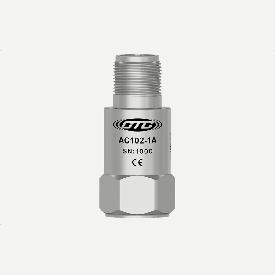
100 mV/g Standard Size Accelerometers
The general-purpose workhorse this post keeps returning to: 100 mV/g on a standard industrial body, with the ±80 g dynamic range that keeps a motor-and-pump route point well clear of the rail. The family spans top-exit, side-exit, M12 and magnet-mount variants, so one sensitivity choice covers a whole route.
- Spectral noise at 1000 Hz
- 2 µg/√Hz
- Sensing structure
- Shear Mode
- Sensing element
- PZT Ceramic
- Constant current excitation
- 2-10 mA
- Bias output voltage
- 10-14 VDC
- Case material
- 316L Stainless Steel
- Maximum shock protection
- 5,000 g, peak
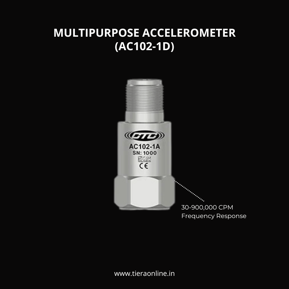
AC102-1D, Multipurpose Accelerometer
The specific unit the TIERA 101 primers teach the datasheet arithmetic from, and the default for a general route point. Top exit, two-pin connector, 100 mV/g at ±10 % — put those into the bench above with a ±5 V rail and you get the fifty-g clip level the worked example uses.
- Sensitivity
- 100 mV/g, ±10%
- Frequency response (±3dB)
- 30-900,000 CPM
- Dynamic range
- ±80 g
- Temperature range
- -58 to 250 °F (-50 to 121 °C)
- Sealing
- Welded, Hermetic
- Connector
- Top exit, 2 pin
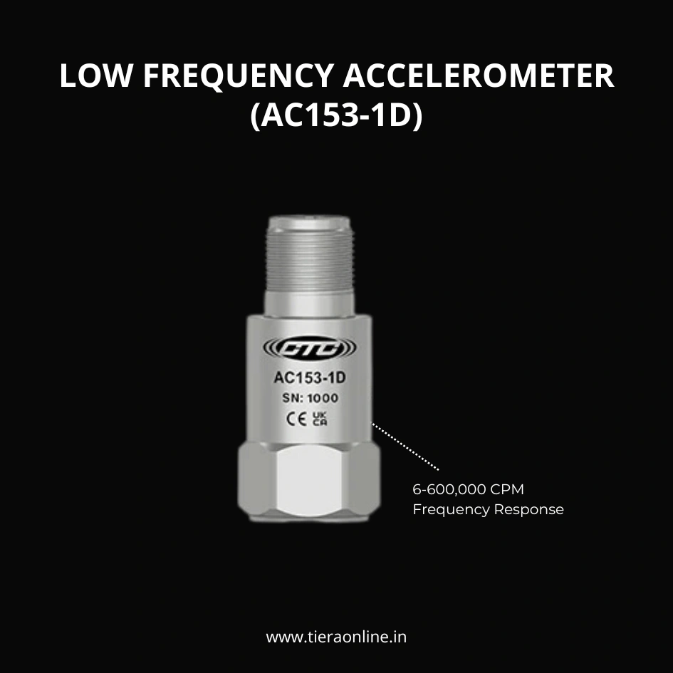
AC153-1D Low Frequency Accelerometer
The slow-machine case from the worked selections: 500 mV/g buys the resolution a twelve-revolution-per-minute agitator needs, and the 6 CPM bottom end reaches down to where its running speed actually sits. Do the clip-level arithmetic before you put this one on anything that impacts.
- Sensitivity
- 500 mV/g, ±15%
- Frequency response (±3dB)
- 6-600,000 CPM
- Designed for
- Low speed rotors, main bearings, gear box inputs
- Temperature range
- -58 to 250 °F (-50 to 121 °C)
- Sealing
- Welded, Hermetic
- Connector
- Top exit, 2 pin
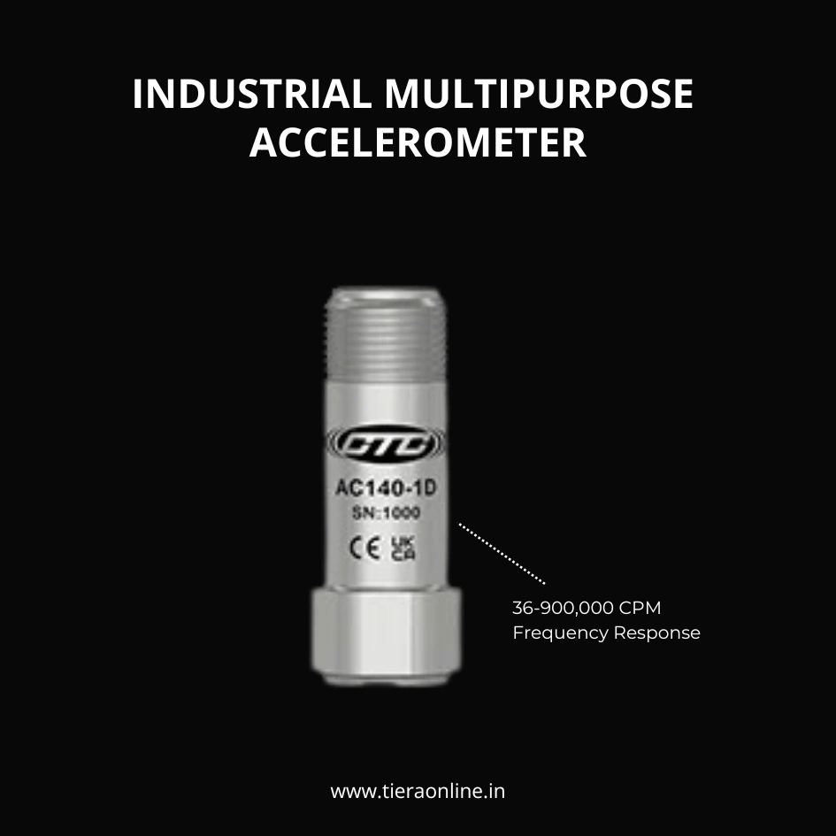
AC140-1D Low Cost Miniature Industrial Multipurpose Accelerometer
The low-mass, hard-to-reach case. When the measurement point is a crowded gearbox housing or a small bearing cap, a miniature body is what lets you get a stud into a prepared face at all — and the stud is what buys the bandwidth a mesh frequency needs.
- Sensitivity
- 100 mV/g, ±15%
- Frequency response (±3dB)
- 36-900,000 CPM
- Suited to
- Hard-to-reach locations
- Temperature range
- -58 to 250 °F (-50 to 121 °C)
- Sealing
- Welded, Hermetic
- Connector
- Top exit, 2 pin mini-mil
From the TIERA store
The kit for this job
What we would actually put in front of someone doing the measurement this post describes — not the whole catalogue.
- 100 mV/g Standard Size AccelerometersCTC's 100 mV/g accelerometers feature high accuracy, low noise, and a wide frequency range, making them ideal for monitoring many industrial applications. The wide frequency response range and ±80 g dynamic range allows these sensors to identify bearing faults at both slower and higher speeds.Request priceView →
- AC102-1D, MULTIPURPOSE ACCELEROMETERMULTIPURPOSE ACCELEROMETER, TOP EXIT 2 PIN CONNECTOR, 100 MV/G, ±10% 30-900,000 CPM Frequency Response (±3dB) -58 to 250 °F (-50 to 121 °C) Temperature Range Welded, Hermetic Sealing CTC’s Best Selling, Multi-Purpose Sensor Ideally Suited for Thousands of Applications₹14,750View →
- AC153-1D LOW FREQUENCY ACCELEROMETERDesigned for low speed Rotors, Main Bearings, and Gear Box Inputs, but may also be used for High Frequency Detection₹34,900View →
- AC140-1D LOW COST MINIATURE INDUSTRIAL MULTIPURPOSE ACCELEROMETERMini Industrial Accelerometer, Great for Hard-to-Reach Locations₹15,000View →
Use cases
Where this shows up in the field
Send us the machine, not the part number
TIERA supplies the industrial accelerometers this post is about, across the sensitivity range it argues over — 100 mV/g general-purpose units for route work, 500 mV/g low-frequency units for slow machines, and miniature bodies for locations where nothing else fits — together with the cables, studs, pads, magnetic mounts and IEPE conditioning that complete the chain.
The more useful thing we can do, though, is the arithmetic in this article on your actual measurement points. Tell us the machine, the peak levels you see at the housing, the highest frequency you need to trust and how you can physically mount on it, and we will tell you which of the three constraints is binding and what fits. Where a figure is not published, ask — and if we cannot give you a measured number for your case, we will say so rather than quote a range.
- 100 mV/g standard-size accelerometers for general route work, 2 µg/√Hz spectral noise at 1000 Hz
- 500 mV/g low-frequency units for slow rotors, main bearings and gearbox inputs
- Miniature industrial bodies for crowded and hard-to-reach measurement points
- Studs, cementing pads, magnetic mounts, cables and IEPE power sources to complete the chain
Where this sits on the TIERA learning ladder.
The theory behind this article is covered free, in full, by the TIERA 101 primers: Accelerometer & DAQ Selection 101, Measurement Setup 101. They are self-paced, interactive, and end in an exam and a certificate.
The free primers work through sensor and DAQ selection and the measurement setup that goes with it; TCAT adds examined, instructor-led depth — reading a calibration certificate, proving a mounted resonance, and defending a measurement chain in a report — with proctored examinations that certify competence.
TIERA 101 is a free introductory primer, not an accredited ISO certification, and its hours do not count towards the formal training ISO 18436 requires.