What a MEMS Noise Floor Costs You, in Detectable Fault Size
Micro-g per root hertz is the least-read line on a wireless sensor datasheet and the one that decides whether it will ever see your bearing fault. Four lines of arithmetic turn it into a fault size in micro-g — with a bench that computes the limit, prices it in seconds of battery, and tells you plainly when the answer is no.
The spec line nobody reads
- Sensitivity is a scaling factor and a gain setting downstream can undo it. Noise density cannot be undone by anything — a tone that reaches the converter smaller than the sensor's own hiss was destroyed inside the sensor, and no filter or model recovers it.
- So the real question is a division, not a technology debate. Its answer is only ever valid for that fault, on that machine, at those settings.
Put a wireless vibration sensor datasheet next to a wired one and most people compare the same three things: the frequency response, the measurement range, and the price. The line that actually decides whether the sensor will find a bearing fault is usually further down, written in a unit nobody uses in conversation: spectral noise density, in micro-g per root hertz. It is the sensor's own hiss, expressed per unit of bandwidth, and it is the floor under every measurement that sensor will ever make.
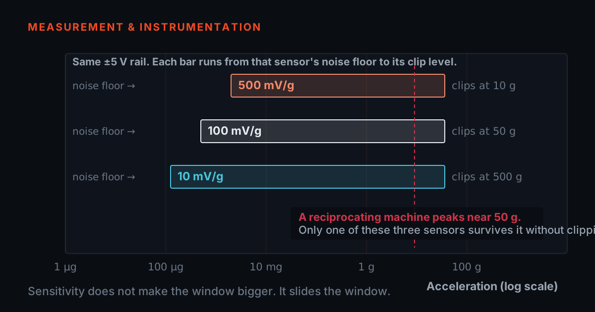
It matters more than sensitivity does, and the reason is worth stating plainly. Sensitivity is a scaling factor — how many millivolts you get per g — and a scaling factor can be undone downstream by a gain setting. Noise density cannot be undone by anything downstream. If a fault tone arrives at the analogue-to-digital converter smaller than the sensor's own noise, the information about that fault was destroyed inside the sensor, before any software existed to be clever with it. No filter recovers it. No machine-learning model recovers it. It is not there.
So the honest version of the question everyone asks — can a wireless MEMS sensor find my bearing fault? — is not a debate about technologies. It is a division. Take the noise density, work out how much of that noise lands in one line of the spectrum, divide by the square root of however many averages you can afford to take, and multiply by whatever signal-to-noise ratio you are willing to call a finding. What comes out is a number in micro-g: the smallest fault tone that sensor can report at those settings. Compare it to the amplitude your fault actually produces, and you have your answer for that fault, on that machine, at that setting — which is the only scope an honest answer has.
This post derives that division, then hands you a bench that runs it. The bench is happy to tell you the answer is no, because on a real programme it sometimes is, and a tool that never says no is not a tool.
Why the grass is lower in a spectrum than in an overall
- A spectral line is a filter one bin wide, so narrowing the bin throws away noise in proportion to bandwidth while the fault tone — being a tone — lands whole inside one line. That asymmetry is why an FFT finds faults an overall reading cannot.
- Resolution is bought with time and instrument capability, not money: a 1 Hz bin needs a one-second record, a quarter-hertz bin four seconds, and 0.25 Hz out to 10 kHz is a forty-thousand-line spectrum most wireless nodes do not offer at all.
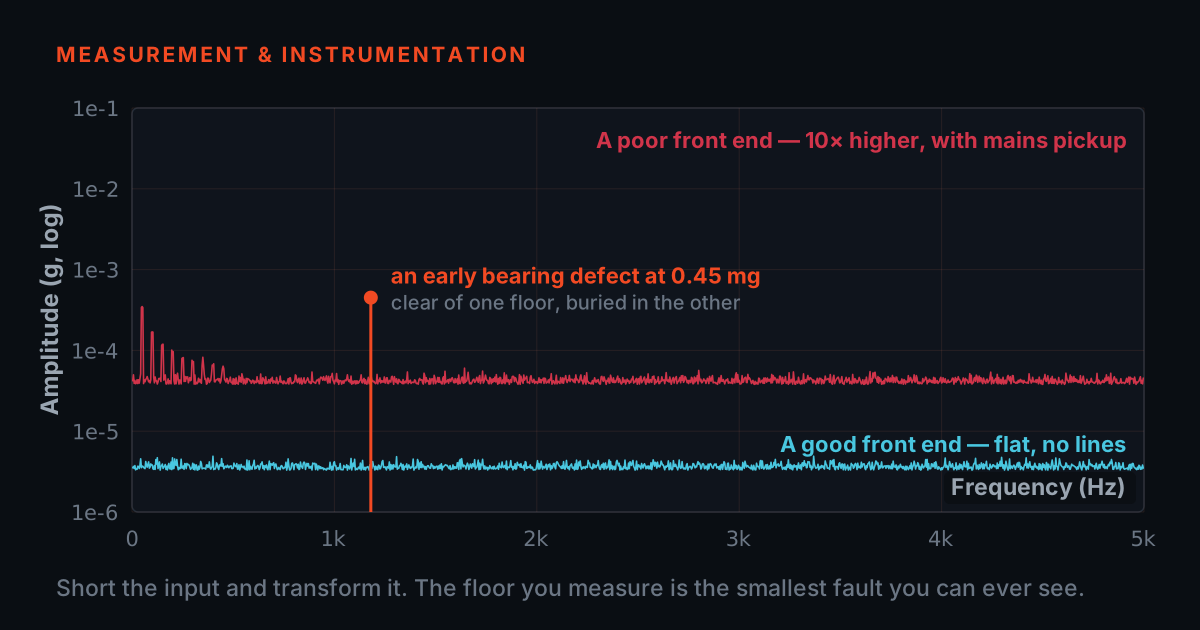
Here is the part that trips up most people the first time, and it is also the reason spectra are worth computing at all. Take a sensor with a noise density of 100 micro-g per root hertz and put it on a machine. Ask it for a broadband overall reading out to 10 kHz and its own noise contributes 100 micro-g times the square root of 10,000 hertz — ten milli-g of pure hiss, before the machine has vibrated at all. Now ask the same sensor, on the same machine, for a spectrum with one-hertz lines. Each line of that spectrum is a filter one hertz wide, so each line collects 100 micro-g times the square root of one: one hundred micro-g. The same sensor. The same noise. A floor one hundred times lower, forty decibels, purely because you looked through a narrower window.
That is the whole reason an FFT finds faults an overall reading cannot. A broadband number sums all the noise in the band into one figure, and it sums the machine's genuine broadband energy in with it. A spectral line sums only the noise that fell inside that line, and the fault tone — which is a tone, concentrated at one frequency — lands entirely inside it. Narrowing the window throws away noise proportional to the bandwidth while keeping the signal intact. That asymmetry is the free lunch, and it is the only one in this article.
It also sets up the trade that runs through the rest of the post. Narrower bins mean a lower floor: halve the bin width and the noise in each bin falls by a factor of the square root of two. But a bin width of one hertz means a record one second long, a quarter-hertz bin means four seconds, and the number of lines the analyser has to compute goes up in step — a quarter-hertz resolution out to 10 kHz is a forty-thousand-line spectrum, which many field instruments and most battery-powered wireless nodes do not offer at all. Resolution is bought with time and with instrument capability, not with money.
MEMS and piezo, honestly compared
A piezoelectric accelerometer generates charge when a seismic mass strains a crystal. A MEMS accelerometer measures the displacement of a tiny silicon proof mass, usually as a change in capacitance, on a die a few millimetres across. They are different devices with different failure modes and different economics, and the useful comparison is not which is better but which line of the datasheet each one wins.
MEMS genuinely wins on several things that matter, and they are not small. It is far smaller and lighter, which means it adds almost no mass to the structure and can go where a piezo body will not fit. It costs an order of magnitude less at the die, which is what makes hundred-point deployments arithmetically possible at all. It runs on microamps rather than needing a constant-current supply, which is the entire reason a battery-powered wireless node can exist. It responds down to DC, so it measures static tilt and true low-frequency motion where an IEPE piezo's own high-pass roll-off has already given up. And it can be embedded — into a motor terminal box, into a gearbox housing, into the sensor node itself — rather than bolted on.
What it gives up is the top and the bottom of the amplitude-and-frequency envelope. Noise floor is the headline: a good industrial IEPE accelerometer publishes single-digit micro-g per root hertz, and the CTC 100 mV/g units TIERA supplies publish two micro-g per root hertz at 1 kHz. Industrial MEMS sits an order of magnitude or two above that, depending heavily on the part — the quietest MEMS parts are genuinely close to piezo, and the general-purpose ones are not close at all. The upper band is the second give: MEMS parts for condition monitoring typically resonate in the low kilohertz, which is why the wireless nodes on this site publish a frequency response to 10 kHz with a plus-nine-and-a-half, minus-six-decibel tolerance and a resonance around five and a half kilohertz — on the Y and Z axes; the triaxial node's X axis is published lower again, to 7 kHz with a 3.5 kHz resonance — rather than the thirty kilohertz a stud-mounted piezo reaches.
It is TIERA's engineering judgement, not a measured claim, that the practical spread across industrial MEMS parts today runs from around twenty-five micro-g per root hertz for the quietest condition-monitoring parts to several hundred for general-purpose ones — and that the difference between two devices both described as 'MEMS' is routinely larger than the difference between the quiet end of MEMS and the noisy end of piezo. That is why the slider below covers three orders of magnitude, and why the only number worth acting on is the one on the datasheet of the specific part, at the frequency it is stated for.
Averaging buys you the square root of n, and only against noise
Linear averaging is the one lever that improves the floor after the sensor has been chosen. Take several spectra of the same steady machine and average them line by line. The machine's tones are in the same place with the same amplitude in every record, so they survive untouched. The noise is random in phase and amplitude, so it partly cancels. The floor drops as the square root of the number of averages — ten log ten of n, which is eighteen decibels for sixty-four averages, and the same eighteen decibels read as an amplitude ratio of eight.
That is a real gain and it is worth taking. It is also the most over-promised idea in condition monitoring, for two reasons. The first is that it only works against random noise. It does nothing for a fixed offset, nothing for a mount that has gone soft, nothing for a fault whose amplitude is genuinely modulating between records, and nothing at all for information the sensor never captured. The second is that it costs time, and the arithmetic is unforgiving: one record at one-hertz resolution is one second, so sixty-four averages is sixty-four seconds of continuous acquisition. On a mains-powered analyser that is a minor inconvenience. On a battery-powered wireless node whose published battery life assumes two short readings a day, sixty-four seconds of radio-on, converter-running acquisition is a design decision with a number of years attached to it.
There is a third trap, and it is quietly the most common. Averaging and resolution pull in opposite directions on the same budget, and they can cancel exactly. Take a hundred micro-g per root hertz sensor with one-hertz bins and no averaging: the limit at a three-to-one call is three hundred micro-g. Now take the same sensor with eight averages — a real improvement, the floor drops by a factor of the square root of eight — but set the analyser to eight-hertz bins to keep the record short. The noise in each bin has gone up by the square root of eight. The two cancel exactly, and the limit is three hundred micro-g again. Both settings are on the bench below as presets, and both print the same number. Nothing was gained; a second of acquisition was traded for nothing at all.
Compute your own detection limit
Everything above is four lines of arithmetic. Here they are as a bench. Set a noise density and a bin width and it computes the noise in one line of the spectrum. Set a number of averages and it lowers that floor by the square root. Set the signal-to-noise ratio you are willing to call a finding and it prints the smallest fault tone those settings can report. Set the amplitude your bearing tone actually produces and it tells you whether you would see it — and how much acquisition time the answer cost.
The machine drawn behind the numbers is fixed speed: 1500 rpm, with an outer-race tone at 107.3 Hz and two of its harmonics. That is deliberate. Nothing in this method requires you to change a machine's speed to make a measurement work, because most plant machines run at one speed and will not oblige. The running-speed line and its second harmonic are drawn as fixed shape rather than as data — they are there so the picture looks like a spectrum, and they are large enough that the noise floor never threatens them. It is the bearing tone that lives near the limit, which is exactly where the real question is.
One behaviour is deliberate and worth watching for. When the tone you asked about falls below the computed limit, the bench does not soften it. It says the sensor cannot report that fault at those settings, and it says why more analysis will not help: the information was lost inside the sensor. Load the 'General MEMS, 500 micro-g per root hertz' preset to see it happen on a case that is otherwise identical to one that worked.
- Noise in one bin, after averaging
- —
- Averaging gain
- —
- Smallest fault you can call
- —
- What it costs to acquire
- —
This is a simulator. The noise in one bin is the density times the square root of the bin width; linear averaging divides that by the square root of the number of averages; the detection limit is the result multiplied by the signal-to-noise ratio you insist on; and one record lasts one divided by the bin width, so the acquisition time is the averages divided by the bin width. Those four lines are the whole model, and they are the same source text the unit tests for this page run against. Everything else on the canvas is drawing: the running-speed line and its second harmonic are fixed shape rather than data, the bearing harmonics fall away at 0.6 and 0.35 of the fundamental as a modelling choice, and the grass is drawn at display resolution with a random spread about the computed level rather than one needle per real bin. Noise densities on the slider are a range for orientation; take the number for a real sensor from its own datasheet, at the frequency the datasheet states it for, because noise density is not flat across the band.
Four worked cases, and the numbers they print
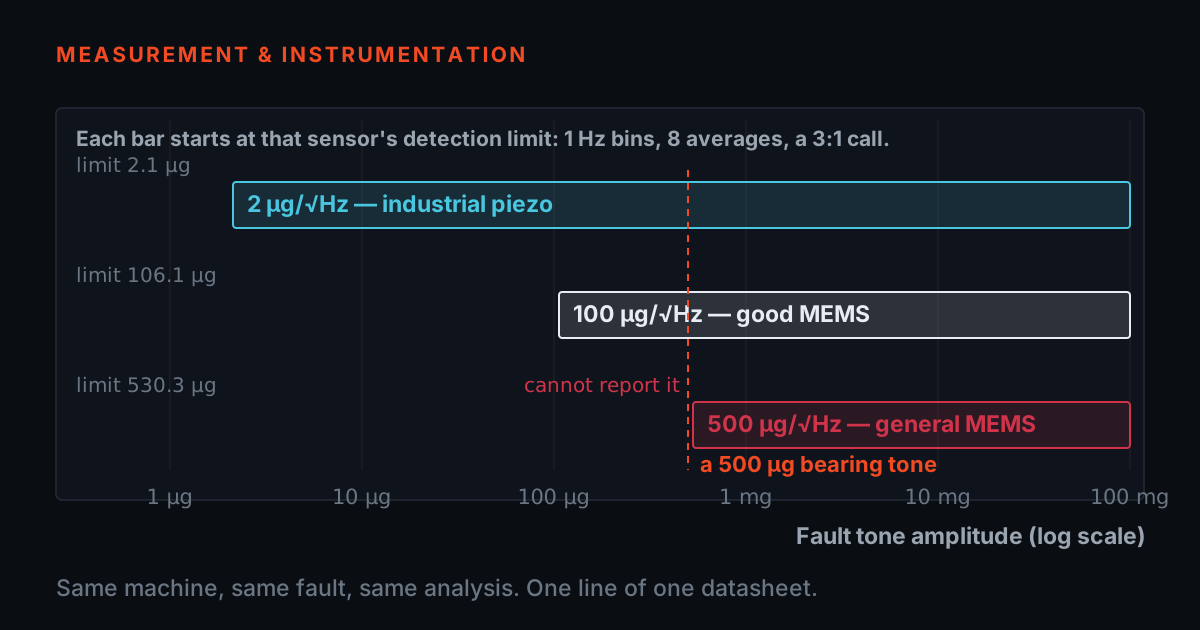
Case one, the reference. A hundred micro-g per root hertz sensor, one-hertz bins, a single record, and a three-to-one call. One hundred micro-g of noise in the bin, no averaging gain, so the limit is three hundred micro-g. A five hundred micro-g bearing tone clears that by 4.4 decibels. It is above the line, and it is still not a finding: grass reaches two to three times its own mean amplitude in the occasional bin, so a peak this close appears in one reading and not the next. This is the case that produces 'intermittent' bearing alarms that nobody can reproduce.
Case two, the wired comparison. Same machine, same tone, same analysis — but a piezo sensor at the two micro-g per root hertz the CTC hundred-millivolt-per-g units publish at one kilohertz, with eight averages. The limit is 2.1 micro-g. The tone stands 47.4 decibels clear. Not marginally better: a different regime entirely, in which the sensor's noise has stopped being part of the conversation and the limiting factor has moved somewhere else — the mount, the cable, the analyser's own front end.
Case three, the honest MEMS answer. A good MEMS part at a hundred micro-g per root hertz, eight averages, one-hertz bins. The limit is 106.1 micro-g and the five hundred micro-g tone clears it by 13.5 decibels. That is a genuine finding from a wireless node, and it is worth being as clear about this as about the failures: for a developed bearing fault on an ordinary machine, a good wireless MEMS sensor is a perfectly real instrument. Case four is the same case with a general-purpose part at five hundred micro-g per root hertz: the limit becomes 530.3 micro-g, the tone at five hundred is half a decibel underneath it, and the fault does not exist as far as that sensor is concerned. Sixty-four averages bring the limit to 187.5 micro-g and recover it — at sixty-four seconds of acquisition per reading, which is the number to take to whoever owns the battery budget.
Notice what changed between case three and case four. Not the machine. Not the fault. Not the mount, the analysis, the software or the analyst. One line of one datasheet, and the fault went from a thirteen-decibel finding to invisible. That is the argument of this whole article, and it is why the spec line nobody reads is the one to read first.
When the wireless sensor genuinely cannot see it
- Three cases return no: a defect tone of tens of micro-g on a large, slow or heavily damped machine; anything living above the sensor's usable band; and a fault that changes faster than the reading interval.
- The third is a sampling-cadence problem, not a noise-floor one, and no better sensor fixes it.
- The response is not to abandon wireless. It is to say what the wireless layer is for and keep a wired route, a portable visit or a permanent point for the machines where the arithmetic says no.
There are cases where the arithmetic returns no and no amount of setting-up changes it, and a supplier who will not name them is not worth listening to. The clearest is early-stage bearing damage on a large, slow or heavily-damped machine, where the defect tone at the housing is tens of micro-g rather than hundreds. Against a general-purpose MEMS floor that tone is not merely hard to see, it is absent, and the first thing the wireless programme will detect is the same fault three months later when it has grown by twenty decibels — which is real detection, just much later than the technology was sold as providing.
The second is anything that lives above the sensor's usable band. Gear mesh tones in the multiple-kilohertz range, the high-frequency ringing that envelope analysis demodulates, blade-pass on a high-speed machine: the wireless nodes on this site publish a frequency response to ten kilohertz with a plus-nine-and-a-half, minus-six-decibel tolerance and a resonance near five and a half kilohertz — and on the triaxial node that figure is the Y and Z axes only, because its X axis is published as 0.5 Hz to 7 kHz with a 3.5 kHz resonance, so the ceiling is not even the same in all three directions on one sensor — and the mount you can actually achieve usually caps the honest band well below any of them. A tone above that ceiling is not measured badly, it is measured as whatever the sensor and mount happen to do there, which is a different thing.
The third is the one that does not show up in any specification: a fault that changes faster than the reading interval. A wireless node taking two readings a day cannot characterise a rub that comes and goes with load, a resonance that appears during a process transition, or a looseness that only knocks on start-up. That is not a noise-floor problem and no better sensor fixes it. It is a sampling-cadence problem, and it is covered in the wired-versus-wireless decision guide rather than here.
In all three cases the useful response is the same, and it is not to abandon wireless. It is to be explicit about what the wireless layer is for — trending the faults it can genuinely resolve, at a cost per point that lets you cover a hundred machines instead of ten — and to keep a wired route, a portable analyst visit, or a permanently-wired point for the machines and the faults where the arithmetic says no. A programme designed around what each layer can actually detect works. A programme sold on the promise that one sensor covers everything produces a filing cabinet of stable trends and a bearing failure nobody saw coming.
Do the division before you buy, not after. It takes a minute, it needs one number off a datasheet, and it is the difference between a monitoring programme and an expensive habit.
TIERA instruments that do this work.
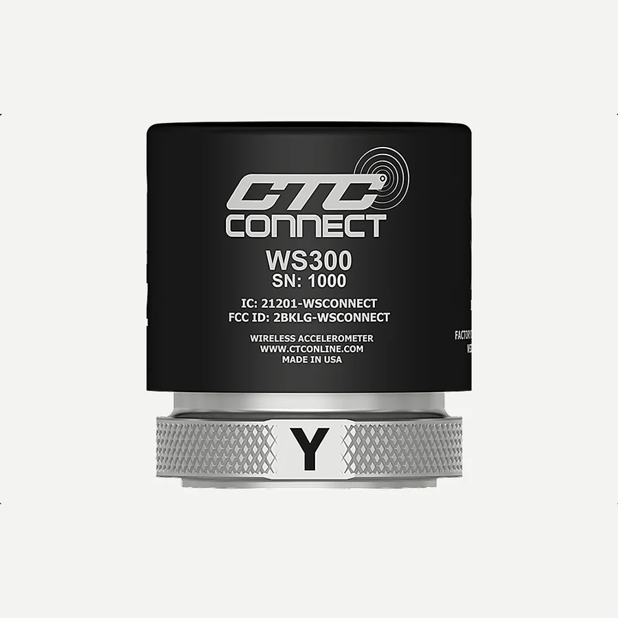
WS300 Series ConnectSens Sensor — Triaxial Dynamic Vibration Signal Capture with Temperature Output
The triaxial wireless node this post's MEMS arithmetic is really about. It returns dynamic vibration samples rather than a scalar, so you get a spectrum to look at in the first place — and its configurable sampling frequency, reading length and dynamic range are exactly the settings the bench above prices. Take its noise density from CTC's own datasheet for the part you order, and run it through the bench before you commit a route to it.
- Sensing structure
- MEMS - triaxial
- Frequency response (Y, Z axes; +9.5/-6 dB)
- 0.5 Hz to 10 kHz (30 CPM to 600000 CPM)
- Frequency response (X axis; +9.5/-3 dB)
- 0.5 Hz to 7 kHz (30 CPM to 420000 CPM)
- Resonant frequency (Y, Z axes; +9.5 dB)
- 5.5 kHz (330000 CPM)
- Resonant frequency (X axis; +9.5 dB)
- 3.5 kHz (210000 CPM)
- Dynamic range
- Configurable: ±8 g, ±16 g, ±32 g, ±64 g
- Sample resolution
- 16 bits
- Expected battery life
- 4 years based on 2 readings taken per day with excellent signal strength at 20 °C
- Wireless protocol
- Bluetooth® Low Energy 5.2
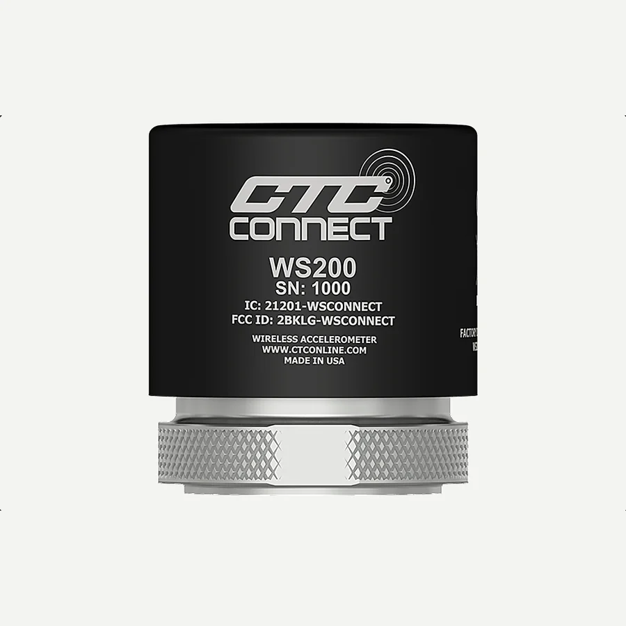
WS200 Series ConnectSens Sensor — Single-axis Dynamic Vibration Signal Capture with Temperature Output
The single-axis version of the same node, for points where one direction is the direction that matters and the budget has to stretch further. Same MEMS sensing structure, same published band and resonance, same configurable record settings — so the same arithmetic applies unchanged, and so does the acquisition-time question the bench raises about deep averaging on a battery.
- Sensing structure
- MEMS
- Frequency response (+9.5/-6 dB)
- 0.5 Hz to 10 kHz (30 CPM to 600000 CPM)
- Frequency response (±10%)
- 0.5 Hz to 1 kHz (30 CPM to 60000 CPM)
- Resonant frequency (+9.5 dB)
- 5.5 kHz (330000 CPM)
- Dynamic range
- Configurable: ±8 g, ±16 g, ±32 g, ±64 g
- Ingress protection
- IP67
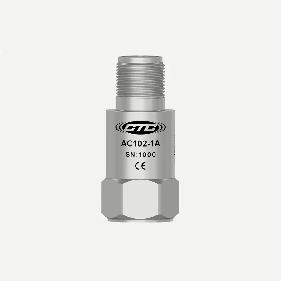
100 mV/g Standard Size Accelerometers
The wired comparison in case two, and the reason the piezo column of the trade figure has a published number in it: two micro-g per root hertz at one kilohertz, printed on the datasheet rather than implied. This is the sensor for the machines and the faults where the wireless arithmetic returns no — early damage, high-frequency evidence, anything that has to be defended in a report.
- Spectral noise at 1000 Hz
- 2 µg/√Hz
- Sensing structure
- Shear Mode
- Sensing element
- PZT Ceramic
- Constant current excitation
- 2-10 mA
- Maximum shock protection
- 5,000 g, peak
- Case material
- 316L Stainless Steel
From the TIERA store
The kit for this job
What we would actually put in front of someone doing the measurement this post describes — not the whole catalogue.
- WS300 Series ConnectSens Sensor - Triaxial Dynamic Vibration Signal Capture with Temperature OutputCTC's WS300 Series ConnectSens™ wireless vibration sensors provide triaxial dynamic vibration signal capture and temperature measurement, offering a versatile solution for predictive maintenance in industrial applications.Request priceView →
- WS200 Series ConnectSens Sensor - Single-axis Dynamic Vibration Signal Capture with Temperature OutputCTC's WS200 Series ConnectSens™ wireless vibration sensors provide single-axis dynamic vibration signal capture and temperature measurement, offering an effective solution for predictive maintenance in industrial applications.Request priceView →
- 100 mV/g Standard Size AccelerometersCTC's 100 mV/g accelerometers feature high accuracy, low noise, and a wide frequency range, making them ideal for monitoring many industrial applications. The wide frequency response range and ±80 g dynamic range allows these sensors to identify bearing faults at both slower and higher speeds.Request priceView →
Use cases
Where this shows up in the field
Tell us the fault you need to catch, and we will do this division with you
TIERA supplies both halves of this trade — CTC's wireless MEMS nodes for scale and coverage, and CTC's industrial IEPE accelerometers with their published noise densities for the points where the arithmetic says a wireless node will not do — along with the mounts, gateways and conditioning that make either of them a measurement rather than a number.
The more useful thing we can do is run this calculation on your machines before anything is ordered. Tell us the fault you are trying to catch, the amplitude it produces at the housing on a machine you have already seen fail, and how often you need to look. We will tell you which points a wireless layer can genuinely cover, which ones need a wired or route measurement, and what the averaging setting costs in battery life. Where a figure is not published for a part, we will say so and ask the manufacturer rather than quote a range.
- CTC ConnectSens wireless nodes returning dynamic vibration samples, single-axis and triaxial
- CTC 100 mV/g industrial accelerometers with 2 µg/√Hz spectral noise published at 1000 Hz
- Mounts, studs, pads and magnets — because the mount caps the band the floor is measured over
- A written detection-limit calculation per measurement point, before you commit to a layer
Where this sits on the TIERA learning ladder.
The theory behind this article is covered free, in full, by the TIERA 101 primers: Accelerometer & DAQ Selection 101, Signal Processing 101. They are self-paced, interactive, and end in an exam and a certificate.
The free primers cover sensor and DAQ selection and the signal processing that turns a record into a spectrum, including where resolution and averaging come from; TCAT adds examined depth — reading a noise-density specification properly, deriving a detection limit for a specific machine, and defending the choice of measurement layer in a report — with proctored examinations that certify competence.
TIERA 101 is a free introductory primer, not an accredited ISO certification, and its hours do not count towards the formal training ISO 18436 requires.