Coherence: the Number That Tells You Your FRF Is Lying
Every FRF comes with a built-in lie detector, and most people never look at it. What coherence actually measures, why it dips at antiresonances but must not dip at your peaks, how H1 and H2 fail in opposite places, and why a single average always reads a perfect — and perfectly meaningless — 1.0.
Divide out the blow: what an FRF really is
- The division only cancels the blow if the force you divided by is the force the structure actually felt — all of it, and nothing else.
- When it is not, the FRF still comes out of the analyser confident and smooth. Nothing on the FRF plot itself will tell you it is wrong.
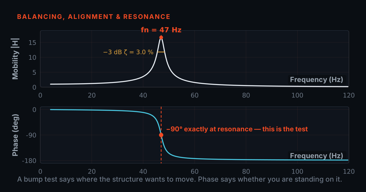
A Frequency Response Function is the response of a structure per unit of input force, frequency by frequency. That 'per unit' is the whole point. Hit a bracket softly and it responds a little; hit it hard and it responds a lot — but divide each response spectrum by its own measured force spectrum and the two results collapse onto one curve. The division cancels how hard you hit, so what remains is a property of the structure: its mass, stiffness and damping arranged along the frequency axis. That is why an FRF measured on Tuesday should overlay one measured on Friday, and why our mode-shapes primer at /blog/modal-testing-mode-shapes can talk about peaks as if they belong to the bracket rather than to the hammer.
But the division only cancels the blow if the force you divided by is the force the structure actually felt — all of it, and nothing else. The moment part of the response comes from something you did not measure (electrical noise, a running machine next door, a rattling joint generating its own excitation), you are dividing apples by half the oranges. The FRF still comes out of the analyser looking confident and smooth. It is simply wrong, and nothing on the FRF plot itself will tell you.
That is the job of the coherence function: the quality metric that ships alongside every averaged FRF, costs nothing to compute, and is skipped by more test engineers than any other number in structural dynamics.
Coherence: how much of the response your force explains
- Coherence is a vote among your averages about whether the input-output relationship held still: agreeing block phasors add into a long resultant, contaminated ones cancel.
- A low value means one of three things — an unmeasured input, mostly noise, or a structure not responding linearly.
- It is not a signal-to-noise meter for one channel and not a smoothness check: a beautifully smooth FRF can carry terrible coherence.
Coherence, written γ²(f), is the fraction of the measured response power that is linearly explained by the measured input, at each frequency, judged across the averaged blocks: γ² = |G̅xy|² / (G̅xx · G̅yy), where G̅xx and G̅yy are the averaged auto-spectra of force and response and G̅xy is their averaged cross-spectrum. A value of 1.0 at some frequency says: every bit of response power there is accounted for, linearly and with consistent phase, by the force you measured. A low value says one of three things — something you did not measure is also moving the structure, or what you recorded there is mostly noise, or the structure is not responding linearly to the force.
The mechanism is worth holding in your head, because it explains everything that follows. Each averaged block contributes a complex cross-spectrum — an arrow with magnitude and phase. If the force truly drives the response through a fixed linear system, every block's arrow points the same way, the arrows add tip-to-tail into a long resultant, and the ratio comes out near one. If noise or an unmeasured input contaminates the blocks, each arrow points a slightly different way, the sum partially cancels, and coherence falls. Coherence is a vote among your averages about whether the input-output relationship held still.
Notice what it is not: it is not a signal-to-noise meter for one channel, and it is not a smoothness check on the FRF. A beautifully smooth FRF can carry terrible coherence, and a jagged-looking FRF at fine resolution can be backed by 0.99 everywhere that matters.
A field guide to coherence dips
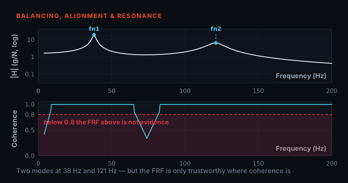
Coherence drops for specific reasons, and each reason has a recognisable shape. Too little excitation energy at a frequency means the tiny genuine response drowns in the noise floor — coherence dips. The classic case is the antiresonance: the structure barely responds there by design of its own dynamics, so a sharp coherence notch sitting exactly in an FRF valley is normal, expected, and no reason to redo anything. The same starvation happens at the top of the band when a soft hammer tip runs out of energy: coherence rolls off smoothly above some frequency, telling you where your usable bandwidth ends.
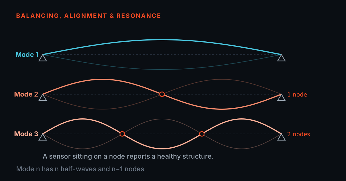
Then there are the sins. A double hit — the hammer bounces and strikes twice — puts comb-shaped notches in the force spectrum; wherever the force dips, coherence dips, so you see evenly spaced coherence notches marching across the band. Leakage from an un-windowed or truncated transient smears energy between bins and shows up as coherence loss concentrated around sharp resonances (our window comparator at /blog/fft-window-comparator shows the smearing itself). Extraneous excitation — a compressor running two bays over — collapses coherence in a narrow band at that machine's frequency and its harmonics, because that part of the response has nothing to do with your hammer. A rattling or nonlinear joint bleeds response energy to frequencies the force cannot linearly explain, dragging coherence down broadly, and it will not average away. A sensor sitting on a node of a mode measures nothing but noise for that mode. And an overloaded channel clips while an under-ranged one quantises — both corrupt the spectra and both leave coherence fingerprints before you would ever spot them on the FRF.
The diagnostic habit, then, is not 'is coherence high?' but 'do I recognise the shape of every dip?'. Antiresonance notches and top-of-band roll-off: expected physics. Combs, narrow collapses at alien frequencies, broadband sag that averaging cannot cure: the test itself needs fixing before the data is worth keeping.
H1 versus H2: two honest estimators, two different lies
- H1 sits below the true curve at the peaks, so it systematically over-estimates damping — which is exactly the quantity you read from peak height.
- H2 props the antiresonance valleys up above the truth. The two bracket the real FRF, and the gap between them is exactly the coherence: γ² = H1/H2.
- Default to H1 for impact testing, and treat any frequency where the two visibly disagree as a frequency where you are choosing between two educated guesses.
With noisy measurements there is no single 'the FRF' — there are estimators. H1 divides the averaged cross-spectrum by the input auto-spectrum (G̅xy/G̅xx); it is built on the assumption that the noise lives on the output channel. Under that assumption the uncorrelated output noise averages out of the cross-spectrum and H1 converges to the truth. But feed it the opposite problem and it fails predictably: at a resonance the response is huge and clean while the force needed to produce it is at its smallest — the structure's impedance collapses, so the force channel is the one working closest to its own noise — and any noise that is actually on the input inflates G̅xx — the denominator — so H1 sits below the true curve exactly at the peaks. Since peak height is what you read damping from, H1 systematically over-estimates damping at resonances.
H2 divides the output auto-spectrum by the cross-spectrum (G̅yy/G̅yx) and assumes the noise is on the input. It is the better choice at resonances, where the force signal is comparatively weak and input noise dominates. Its own failure lives at the antiresonances: there the response is tiny, output noise inflates G̅yy — now the numerator — and H2 props the valley up above the truth. The two estimators bracket the true FRF: H1 from below, H2 from above, and the gap between them at any frequency is, not coincidentally, exactly the coherence: γ² = H1/H2. When coherence is 1, the estimators agree and there was nothing to argue about.
The practical consequence, without the derivations: use H1 as the default for impact testing (output noise is the common case), glance at H2 — or the H1/H2 gap — when peak amplitudes and damping matter, and treat any frequency where they visibly disagree as a frequency where you are choosing between two educated guesses. TVIB's TSAP201 computes both estimators and flags coherence below your acceptance threshold, which turns this whole judgement into a visible, per-measurement check rather than folklore.
The one-average trap: why γ² = 1 can mean nothing
Here is the fact that catches more beginners than any other in FRF work: computed from a single block, coherence is identically 1.0 at every frequency, always, regardless of how bad the data is. This is not a software quirk. With one block, |Gxy|² equals Gxx·Gyy as a mathematical identity — one arrow cannot disagree with itself. Coherence measures consistency between averages, so with nothing to compare, the ratio degenerates to perfection. A perfect coherence trace over a single hit is the instrument politely reporting that it has no information yet.
This is why averaging several impacts is not just noise reduction — it is what makes the quality check exist at all. Three to five averages give coherence its first real meaning; eight to sixteen is a comfortable working range for impact testing, and more buys diminishing returns unless coherence is marginal. Each extra block is another independent witness asked the same question: did this force produce this response? Averaging also reduces the random error of the coherence estimate itself, so a dip you see at N = 16 is believable in a way the same dip at N = 3 is not.
The corollary is a habit: distrust any FRF delivered without its coherence trace and its average count. 'Coherence was 1.0' is only praise if N was greater than one — otherwise it is a confession.
Try it: watch coherence collapse and recover
The instrument below is real, not an illustration. It synthesises a two-mode structure (modes at 45 and 120 Hz with an antiresonance between), fires a fresh set of simulated hammer blows — each with its own strength, timing and noise — and accumulates the auto- and cross-spectra over the number of averages you choose. H1 and coherence are then computed from those averaged spectra, exactly as an analyser does it. Nothing is drawn from a lookup table, which is why the one-average identity falls out on its own: slide averages down to 1 and watch coherence snap to a flat, useless 1.0.
Then break the measurement on purpose. Raise the response-channel noise and watch coherence sag first at the antiresonance, at the very bottom of the band and at the top of it — the three places where the genuine response is smallest, because an accelerance FRF falls away below the first mode just as surely as the hammer runs out of energy above the last one — while the peaks themselves hold firm. Switch on the double hit and comb notches appear where the force spectrum self-cancels. Set the nearby machine running and coherence collapses in narrow bands at 30, 60 and 90 Hz that have nothing to do with your structure. In every case, watch how many averages it takes for the verdict card to stabilise.
The honest reading rule — and a representative rescue
The rule that separates professional FRF work from hopeful FRF work: judge coherence at the frequencies you intend to use, not on average. A trace that averages 0.97 across the band tells you almost nothing; a trace that reads 0.99 on the two peaks you are about to extract damping from tells you everything. Symmetrically, a coherence crater at an antiresonance is expected physics and invalidates nothing — while a low-coherence patch sitting on a resonance peak invalidates that mode, however pretty the peak looks. One number per peak-of-interest, checked before the hammer goes back in the case: that is the whole discipline. Once a mode is validated, whether your machine's running speed can reach it is the interference story we tell in the Campbell explorer at /blog/campbell-resonance-explorer.
A representative test, not a specific customer: a two-day modal survey of a pump skid produces textbook FRFs, but the coherence trace shows a hard notch at 24.8 Hz — directly under the first bending mode the survey exists to find. Averaging more hits does not lift it, which rules out random noise. A glance across the bay finds a cooling-tower fan turning at 1,488 RPM: 24.8 Hz, an unmeasured input feeding the response channel at exactly the wrong frequency. The fan is locked out for twenty minutes, six fresh averages are taken, coherence at the mode comes up to 0.995, and the extracted damping ratio changes by a third against the contaminated set — the difference between a defensible result and a plausible-looking fiction. Total cost of the check: one glance at a trace the analyser was already computing.
If the concepts here moved faster than you would like, the free primers at 101.tieraonline.in — start with Modal & Resonance 101 — build up FRFs, resonance and mode shapes at beginner pace; they are open primers, not accredited ISO certification. For formally assessed analyst competence, TIERA's TCAT programme (details at /services) adds structured coursework with proctored examinations at exams.tieraonline.in.
TIERA instruments that do this work.

PhonoVibe Series — Sound & Vibration DAQ
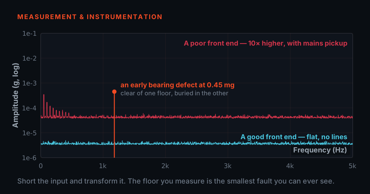
Coherence is only meaningful if force and response are captured on the same clock — PhonoVibe samples every input simultaneously at 24 bits, so the cross-spectrum phase is real, not an artefact of channel skew.
- ADC resolution
- 24-bit across the entire series
- Sampling
- Simultaneous on every input; up to 128 kHz (Q/O/HD)
- Channels
- 2 / 4 / 8 / 16 (D, Q, O, HD)
- Sensor power
- IEPE / ICP / CCLD — 24 V, 4 mA constant current
- TEDS
- Supported

TVIB — Sound & Vibration Analysis Software
TSAP201 computes H1 and H2 FRF estimators and flags any measurement whose coherence falls below your acceptance threshold — the workflow this whole post argues for, built into the capture screen.
- FRF & modal
- TFRT FRF module + TIST 205 modal pre-processing
- Averaging
- Exponential, linear, peak hold, with selectable windowing
- FFT size
- Up to 102,400 points
- Base module
- TSAP201 — free with every PhonoVibe DAQ
- Trial
- 14-day fully-unlocked evaluation licence
TWGM 206 — Waveform Generator
When impact testing cannot deliver clean coherence, shaker excitation can: burst signals that start and end inside the record kill leakage, and the bandpass option keeps energy inside the band you are measuring.
- Noise signals
- Pink, white, and random noise generation
- Burst excitation
- Noise burst and sine-sweep burst for FRF averaging
- Sweeps
- Linear and logarithmic sine sweep
- Band control
- Bandpass filter on noise output limits energy to the measurement bandwidth
- Drives
- T-Xcite series electrodynamic shakers and amplifiers, via PhonoVibe DAC
From the TIERA store
The kit for this job
What we would actually put in front of someone doing the measurement this post describes — not the whole catalogue.
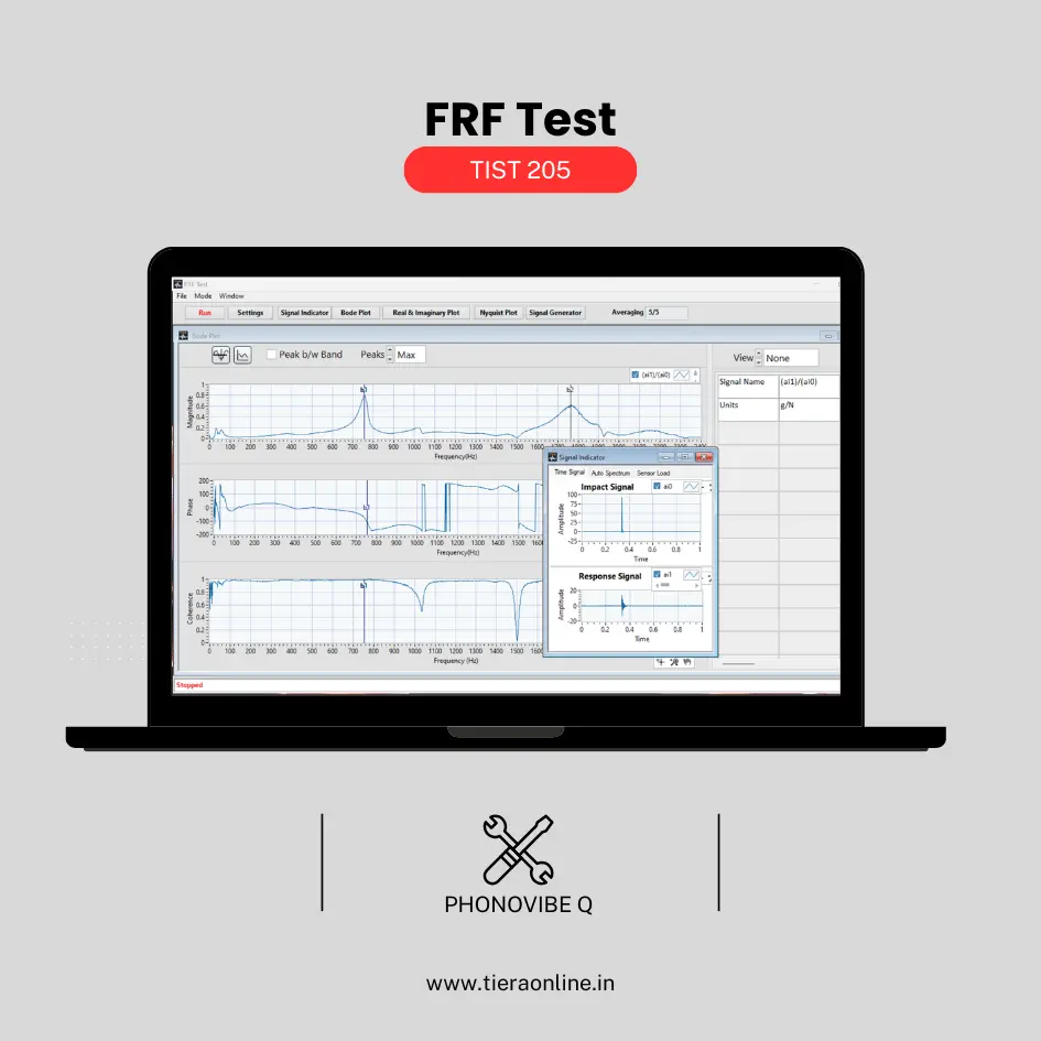 TIST 205 – FRF Test (Phonovibe Q)Use Cases Experimental Modal Analysis Product quality Natural Frequency Transmissibility,Vibration isolation Measurement₹41,472View →
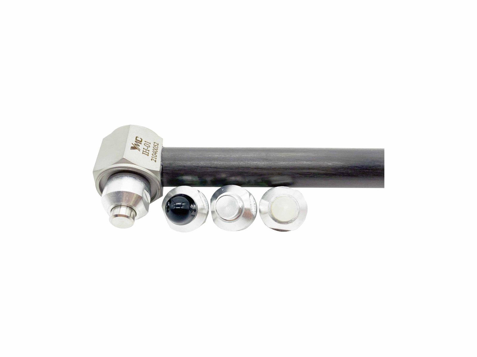 Impact Hammer-IH-01A rugged force sensor built into the hammer’s striking surface. A variety of hammers are suitable for different size test subjects. Tips offer a frequency-tailored impulse. Used for structure health testing, resonance determination, modal analysis.₹67,000View →
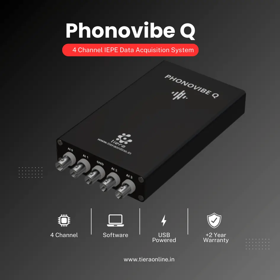 4 Channel IEPE Data Acquisition System – Phonovibe QFour Channels Standard plug & play USB Powered Take data from accelerometers, microphones, hammers, or any other IEPE Sensors T- VIB Software to acquire time waveforms, frequency spectra, overall vibration levels, FRF’s and octave measurements ** Windows 10 or above Operating System ** T-VIB Software base version comes with Time and Spectrum with Post processor TSAP 201. Check out TVIB Software regarding more module options.₹2,88,000View →
Use cases
Where this shows up in the field
A measurement chain where the lie detector is on by default
Everything in this post assumes your acquisition chain can be trusted to tell you when it can't be trusted. PhonoVibe DAQs capture the force and every response channel simultaneously on 24-bit converters with IEPE sensor power and TEDS recognition, so the averaged cross-spectra that coherence is built from reflect the structure, not channel timing. TVIB's TSAP201 — bundled free with every PhonoVibe — computes H1 and H2 estimators side by side and flags measurements whose coherence falls below your acceptance threshold before they contaminate a modal data set.
When hammer excitation can't deliver coherent data — lightly damped modes, big structures, stubborn noise floors — the TWGM 206 generator supplies burst-random and burst sine-sweep signals straight from the PhonoVibe's DAC into T-Xcite shakers and amplifiers, with a bandpass option that concentrates energy where you are actually measuring, while TIERA's shaker stands hold the excitation geometry repeatable between runs.
- PhonoVibe D / Q / O / HD — 2 to 16 channels, 24-bit, simultaneous sampling with IEPE power and TEDS, so cross-spectrum phase is measurement, not skew
- TVIB TSAP201 + TFRT — H1/H2 FRF estimators with coherence flagged against your acceptance threshold, plus exponential / linear / peak-hold averaging
- TWGM 206 — noise bursts and sine-sweep bursts for leakage-free averaged FRFs, bandpass-limited to the measurement band
- Vertical and lateral shaker stands — repeatable vertical, horizontal and oblique excitation so a coherence problem is never a fixture problem
Where this sits on the TIERA learning ladder.
The theory behind this article is covered free, in full, by the TIERA 101 primers: Modal & Resonance 101. They are self-paced, interactive, and end in an exam and a certificate.
The free Modal & Resonance 101 primer at 101.tieraonline.in covers FRFs, resonance and mode shapes at beginner pace; the formal TCAT programme (see /services) adds structured analyst coursework with proctored, exam-verified certification at exams.tieraonline.in.
TIERA 101 is a free introductory primer, not an accredited ISO certification, and its hours do not count towards the formal training ISO 18436 requires.