Published · Updated
Your Envelope Band Is Perfect. Your Sensor Can't Reach It.
A boiler feed pump destroyed a bearing three weeks after a route that read perfectly clean. Nothing was wrong with the analysis. Everything was wrong with the instrument. Four simulators take the failure apart — reach, noise floor, headroom and the loop — across the eight IMI precision ICP accelerometers.
Act I · A bearing that failed three weeks after a clean route
The machine is a boiler feed pump: 200 kW, 1,440 rpm, 24 Hz at the shaft, with a 6316 deep-groove ball bearing at the non-drive end. Outer-race defect frequency, 74 Hz — eight balls, 28.6 mm on a 125 mm pitch circle, so just over three times shaft rate. It sat on a monthly vibration route for four years without incident.
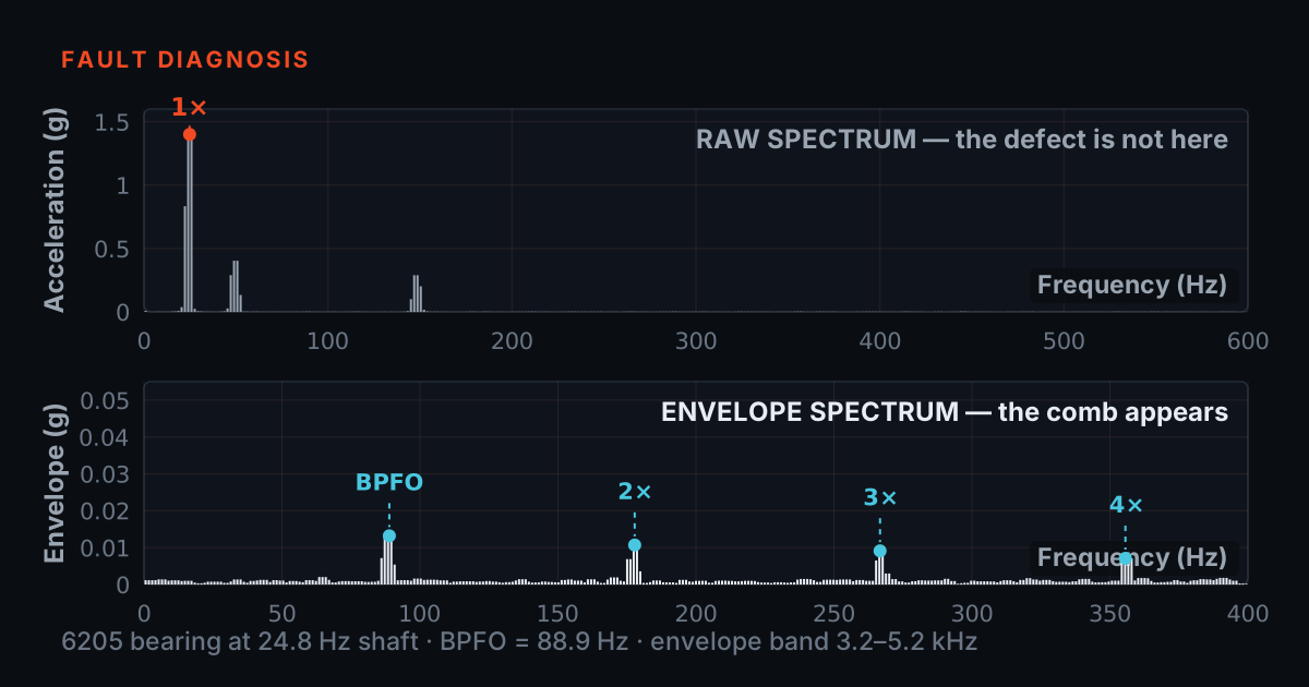
On the March route it read clean. Overall velocity 2.1 mm/s RMS, comfortably in ISO 20816 Zone A. The spectrum showed 1× shaft, a little 2×, vane pass, nothing else. The analyst signed it off, correctly, on the evidence in front of him.
Twenty-three days later the bearing seized. The strip-down found an outer-race spall roughly 9 mm across with established secondary damage around it — a defect that does not appear in three weeks. It had been growing for the better part of a year, through eight monthly routes, every one of which read clean.
The obvious conclusion is that somebody missed it. The obvious conclusion is wrong. Nobody missed it, because it was never in the data. The envelope band was tuned correctly, the analysis was competent, and the defect was physically incapable of reaching the analyser — for three separate reasons, each of which is printed on a datasheet nobody had read.
Act I · Three gates stood between the spall and the spectrum
- An envelope band is a request. The accelerometer is what answers it — and the usual teaching assumes the signal arrives at the analyser at all.
- Reach, noise floor, headroom. Three gates, all printed on the datasheet, and all decided at the purchase order rather than in the analyser.
Two earlier posts on this blog take the technique apart. Why a Failing Bearing Hides in the Noise explains the physics: a spall is a tiny, perfectly repetitive impact that rings the housing at a few kilohertz, and enveloping recovers its rhythm by band-passing that ringing and rectifying what is left. Tune the Band, Find the Bearing makes it a tuning exercise you can drive: park the window on the resonance and the comb appears; slide off and it vanishes.
Both posts quietly assume something that was false on this pump. They assume the signal reaches the analyser.
An envelope band is a request. The accelerometer is what answers it. If the housing rings at 6 kHz and the sensor is specified flat to 10 kHz but resonates at 18 kHz, you are working where the sensor is already inflating your amplitudes. If the spall puts 300 µg of ringing into the housing and the sensor's own electrical noise contributes 330 µg across the same band, no tuning on earth finds the comb — you would be demodulating the amplifier. And if the machine hammers hard enough to drive a ±50 g sensor into its stops, the clipping manufactures a comb of its own, at frequencies that have nothing to do with the bearing.
Reach, noise floor, headroom. Three gates, all decided before anyone opens the analyser, all printed on the datasheet. Act II takes them one at a time against a real product line — the IMI Sensors precision ICP range, eight series from the 621 to the 628 — and gives you an instrument for each.
Act II · Gate one — could the sensor reach the ring?
- Mounted resonance is where the sensor peaks; the ±3 dB corner is where the manufacturer will still guarantee the amplitude. The 623 resonates at 40 kHz and is specified only to 15 kHz.
- Between the two the sensor still produces output — often a great deal of it — but it is no longer calibrated. It will find a defect; it will not tell you how big the defect is.
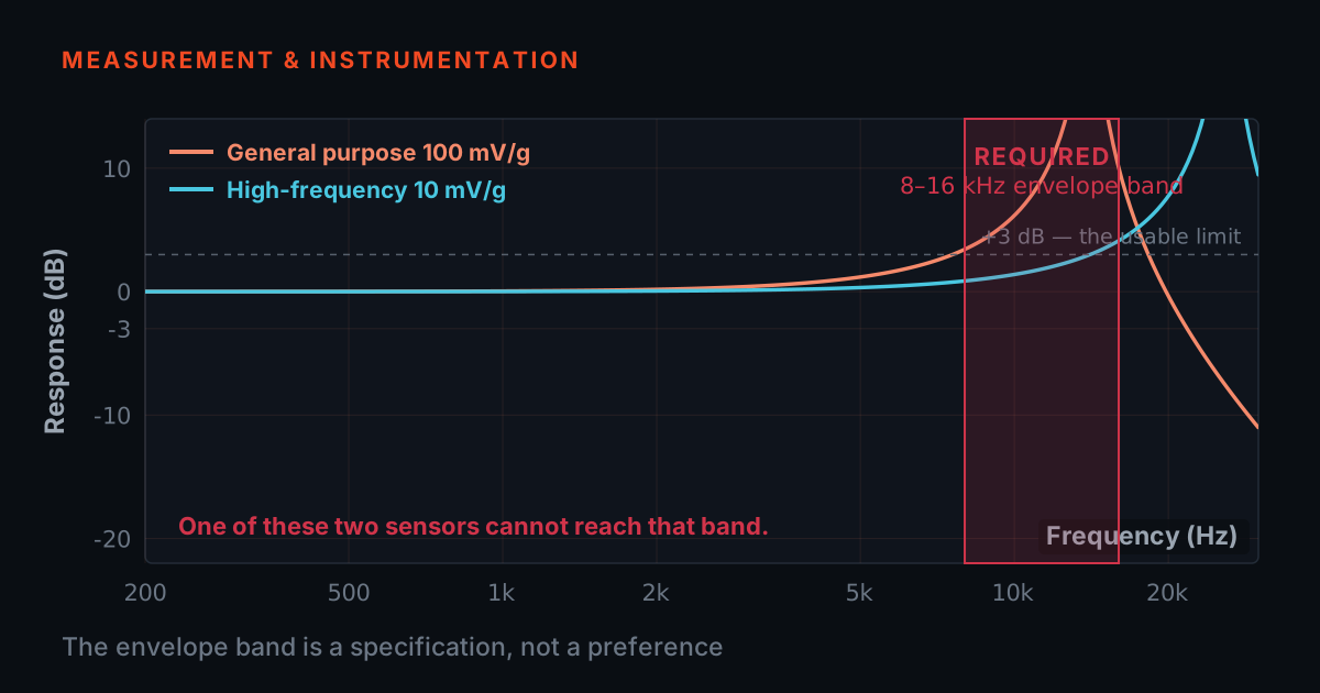
- The three quartz units all resonate at 18 kHz and are specified to 10–12 kHz, so their rise begins exactly where the envelope band lives.
A rolling-element defect does not radiate at its defect frequency. It radiates a short impulse, and that impulse excites whatever structural resonance is nearest — the bearing outer ring, the housing, the sensor's own mounted resonance. In industrial machines that ringing typically lands between 2 kHz and 20 kHz. Enveloping works precisely because that band sits far above the shaft and blade energy that swamps the low end.
So the sensor has to be honest up there. A piezoelectric accelerometer is a mass on a spring: below its mounted resonance it is flat, approaching resonance it lifts, past resonance it collapses. That is why the datasheet prints two different numbers, and confusing them is the most common selection error in the field.
Mounted resonance is where the sensor peaks. The ±3 dB corner is where the manufacturer will still guarantee the amplitude. They are not the same, and the gap is large: the 623 Series resonates at 40 kHz but is specified only to 15 kHz. Between the two it still produces output — often a great deal of it — but that output is no longer calibrated. It will find a defect. It will not tell you how big the defect is.
Plot the range against the band enveloping actually uses and the ranking falls out. The three quartz units — 624, 627, 628 — all resonate at 18 kHz and are specified to 10–12 kHz, so their rise begins exactly where the envelope band lives. The 623 (40 kHz) and 621 (85 kHz) stay genuinely flat across the whole of it.
Act II · Gate two — the arithmetic nobody does
- Noise in band = spectral density × √bandwidth. Across a typical 3,000 Hz envelope window the 622 gives 22 µg and the three quartz units give 329 µg — a factor of fifteen, 23.5 dB.
- A spall putting a couple of hundred µg of ringing into the housing is an obvious comb on one sensor and literally below the noise on another. Same machine, same band, same analyst.
- The 621 has the worst noise floor of the eight — 548 µg in the same band. Its bandwidth and range were bought with sensitivity.
This is the gate that killed the pump, and it is the one almost never checked, because it needs one line of arithmetic the datasheet does not do for you.
Every accelerometer's built-in amplifier contributes noise. The datasheet gives it as a spectral density — µg per root hertz — at 10 Hz, 100 Hz and 1 kHz. A density is not a level. To find out how much noise you actually get, integrate it across the bandwidth you are using. For a flat density that is simply:
noise in band = density × √bandwidth
An envelope band is wide by design — you want the whole resonance, so 2,000 to 4,000 Hz is typical. Take 3,000 Hz and run the eight models through it, using each one's density at 1 kHz, the right figure for a band sitting in the kilohertz region.
The spread is brutal. The 622 delivers 22 µg of noise across that band. The three quartz units deliver 329 µg — fifteen times more, 23.5 dB. An incipient outer-race spall putting a couple of hundred µg of ringing into the housing is a clean, obvious comb on the 622 and is literally below the noise on the 627. Same machine, same analyser, same perfectly tuned band, same analyst, opposite conclusions.
The pump had a 627 fitted. It had been specified years earlier, correctly, for its long-term stability in a hot pump house — and then quietly asked to do a job it was never built for.
There is a second surprise in the table, and it is the honest thing to say about the sensor with the best bandwidth. The 621 has the worst noise floor of the eight. Its 10 mV/g sensitivity buys the ±500 g range and the 85 kHz resonance, and pays for them with 10 µg/√Hz — 548 µg in our band, worse even than the quartz units. The 621 is not the answer to "find me a faint bearing defect." It answers a different question, which is Gate 3.
Act II · Gate three — and the comb that was never there
Gates 1 and 2 push you toward a sensitive, low-noise, high-resonance sensor. Gate 3 pushes back, and on some machines it wins outright.
Seven of the eight models are ±50 g full scale. That is generous for a motor or a pump and not remotely generous for a hammer mill, a reciprocating compressor, a crusher, or a gearbox under shock load. Drive a ±50 g sensor past its range and it does not saturate quietly. It clips — and a clipped waveform is rich in harmonics that were never in the machine.
The simulator below computes this rather than asserting it. It synthesises a machine with a large 1× shaft vibration and an optional bearing defect, hard-clips the waveform at the selected sensor's full scale, then runs a real band-pass, a real Hilbert envelope and a real 4,096-point FFT of that envelope — the same chain an analyser runs.
Set the defect to zero and raise the 1× level past ±50 g. A comb appears. It is not at BPFO; it stands at twice shaft rate and its harmonics, because hard clipping puts a sharp corner into the waveform twice per revolution and the envelope detector reads those corners as impacts. There is no bearing fault anywhere in the signal. Switch the sensor to the ±500 g 621 and the comb vanishes — proving it was the instrument, not the machine.
Then set a real defect and clip it. Two things happen at once, and the second is the one that costs money: a false comb appears at 2× shaft, and the real BPFO comb is suppressed, because flat-topping compresses exactly the impact peaks the envelope is measuring. Clipping invents a fault and understates the real one in the same record.
The pump: 1,440 RPM (24 Hz shaft), 6316 bearing, BPFO 74 Hz, housing ringing near 3 kHz. Record: 4,096 samples at 8,192 S/s. Band-pass 2–4 kHz, Hilbert envelope, 4,096-point FFT — all computed live in your browser.
Act II · The instrument that settles all three gates
Each gate is one calculation, so here they are as a single instrument. Pick a sensor, describe the machine and the mount, and watch all three verdicts move together.
The response curve is computed from each model's published mounted resonance as a single-degree-of-freedom system, with the mount cascaded on top. The noise line is that model's published 1 kHz density integrated across the band width you choose. The envelope spectrum at the bottom is drawn relative to that noise floor — so when the comb sinks into the grass, it is sinking into this specific sensor's grass, for the reason named in the panel.
Three things worth trying. Leave the ring frequency at 3.5 kHz on a stud mount and step through all eight models: the response curve barely moves, and the SNR readout alone swings from +22.7 dB on the 622 to +15.7 dB on the 623, −0.8 dB on the 627 and −5.2 dB on the 621. Same machine, same band, same fixture — Gate 2 decides the entire outcome by itself. That single readout is the pump's whole story.
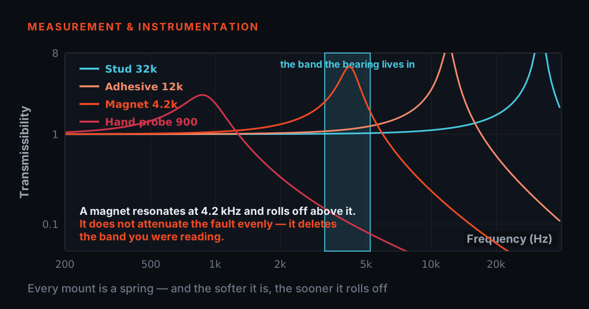
Then leave the 622 selected and switch the mount from stud to magnet, and watch something genuinely counter-intuitive. The SNR gets better — from +22.7 dB to +32.1 dB — because at 3.5 kHz you sit just below the magnet's own 4.2 kHz resonance and it is handing you 9.5 dB of gain. Gate 1 turns amber anyway, and it is right to: that gain is not calibrated, it moves with every remount, and the amplitude you trend has become a property of the magnet. Now drag the ring frequency upward and watch the same fixture turn on you — the mount contributes −8.5 dB at 8 kHz, −17 dB at 12 kHz and −27 dB at 20 kHz, and Gate 1 goes red the moment you pass its 4.2 kHz resonance.
Finally set the transient to 200 g and watch seven of the eight models fail Gate 3 at once, leaving the 621 — the model with the worst noise floor in the range — as the only one that can take the measurement at all.
Bearing: outer-race defect, BPFO = 74 Hz — the pump from Act I, and the same case as the tuning simulator. All eight models carry their published brochure specifications.
GATE 1 · REACH
——GATE 2 · NOISE FLOOR
——GATE 3 · HEADROOM
———
Act III · How much warning does each sensor buy?
Decibels are an abstraction. A maintenance manager does not buy decibels; they buy time — the interval between the first credible warning and the outage. That interval is what the noise floor actually sets, and it is straightforward to compute.
Bearing defect energy grows roughly exponentially once a spall initiates. Give a degradation curve a starting level and a failure level, and each sensor's detection threshold — its own in-band noise, times whatever confidence margin you require — intersects that curve at a different date. The gap between that date and failure is the warning time you have bought.
The instrument below does exactly that. It is the same arithmetic as Gate 2, replotted against a calendar instead of a spectrum.
On the default settings the answer is stark. The 622 raises a credible flag with something over a year in hand. The 627 that was actually fitted to the pump gets there months later — and on a machine whose degradation runs faster than this one, "months later" becomes "three weeks before it seizes", which is precisely what happened.
Two honest caveats sit on this chart, and both are stated on it. Real degradation is not a clean exponential — bearings plateau, and a self-honing spall can look like recovery for weeks. And detection is not the same as diagnosis: crossing the noise floor makes the comb visible, not yet trendable. Both push the real warning time down from what the model says, which is the safe direction for a chart used to justify a sensor.
Defect energy in the resonance band grows exponentially from onset to failure. Each sensor is flagged when the growing signal first exceeds its own in-band noise by the confidence margin you set.
| SENSOR | IN-BAND NOISE | FIRST DETECTED | WARNING |
|---|
Act III · The loop between the sensor and the analyser
- Bias voltage is a free diagnostic almost nobody reads: mid-rail is healthy, at the supply rail is an open circuit, on the floor is a short, and wandering low is moisture in a connector.
- The constant current and the cable capacitance together set a hard frequency ceiling, and it can land below the bearing's ring.
- A long cable run is a bandwidth decision, not a convenience one.
There is a fourth failure that belongs with the other three, because it also caps your bandwidth and it also never appears in an analysis review. It is the two-wire loop itself.
Every model in this range is an ICP® sensor: a constant-current, two-wire system with a built-in amplifier. The brochure sets out the operating conditions precisely. An 18–30 VDC supply feeds a current-regulating diode that holds the line between 2 and 20 mA, dropping about 1 V across itself. The sensor's amplifier sits on that current and produces a DC bias voltage, normally 8 to 12 VDC, with the AC vibration signal riding on top. A 10–30 µF decoupling capacitor at the conditioner strips the DC away so the analyser sees only the signal.
That bias voltage is a free diagnostic and almost nobody reads it. A healthy sensor sits mid-rail. An open circuit — a broken conductor, a connector backed out, a sensor not fitted — lets the bias float up to the supply rail. A short to shield pulls it to zero. Moisture in a connector drags it down and makes it wander. You can tell all of this from a single DC measurement before you record anything.
The second thing the loop decides is more surprising, and it matters directly to everything above: the constant current and the cable capacitance together set a hard ceiling on frequency, and that ceiling can land below the bearing's ring. Driving cable capacitance at high frequency and high amplitude requires current, and an ICP sensor has only what the conditioner supplies minus roughly 1 mA for its own bias:
fmax = 109 × (Ic − 1) / (2π C V) — with Ic in mA, C the total cable capacitance in pF, and V the peak signal in volts.
Work it through. A 4 mA conditioner, 100 m of cable at 100 pF/m and a 5 V peak signal gives 9.5 kHz — enough for a 3.5 kHz housing resonance, not enough for the top of the band. Drop the conditioner to the 2 mA minimum and the same run gives 3.2 kHz, which lands directly on the resonance you were trying to measure. Take a 200 m run of 150 pF/m cable at 2 mA with an 8 V signal and you are down to 660 Hz: the enveloping band is simply absent, and the spectrum will look perfectly plausible while it is missing.
It works the other way too. Raise the conditioner to 10 mA on that 100 m run and you reach 28.6 kHz; shorten the run to 10 m at 4 mA and you are at 95 kHz, far beyond any sensor in the range. This is exactly why the brochure specifies 2 to 20 mA rather than a single value — and why a long cable run is a bandwidth decision rather than a convenience one.
ICP® two-wire loop, per the brochure's operating conditions: 18–30 VDC supply, 2–20 mA constant current through a regulating diode (about 1 V drop), sensor bias normally 8–12 VDC.
BIAS VOLTAGE
——CABLE FREQUENCY CEILING
——Act III · Which one, for which job
- There is no best accelerometer here, only a best fit: the 623 as the default, the 622 when the defect is faint, the 621 when the machine hammers, quartz when the environment is the problem.
- Four of the eight are genuinely good enveloping sensors, three are excellent sensors for a job that is not enveloping, and one is the shock specialist. A range is not a ladder.
Run the gates across the range and the eight series sort into four honest answers rather than a ranking. There is no best accelerometer here, only a best fit — and the quartz units are not the losers of this comparison. They are the answer to a question the pump was not asking.
The default for bearing enveloping: 623. A 40 kHz mounted resonance keeps it flat through the whole practical ringing band, 0.9 µg/√Hz gives 49 µg across a 3 kHz window, and at 51 g and 17.3 mm diameter it fits pump and motor housings where bigger ring-style bodies will not go. It clears Gates 1 and 2 together without an argument.
When the defect is faint: 622. The lowest noise floor in the brochure — 0.4 µg/√Hz at 1 kHz, 50 µg broadband — buys the earliest possible detection, which is the entire point of a trending programme and precisely what the warning-time chart above prices. You trade the 623's resonance headroom (30 kHz rather than 40 kHz) for roughly 7 dB of visibility. On a machine ringing at or below 5 kHz that is a straight win. The 625 is the same argument in a side-exit ring-style body when cable routing is tight, at 0.5 µg/√Hz.
When the machine hammers: 621. ±500 g, a 10,000 g shock limit, ±3 dB to 30 kHz and 4.75 grams. Gate 3 overrules Gates 1 and 2 on crushers, mills, reciprocating machines and shock-loaded gearboxes, because a clipped record is not a worse measurement — the clipping simulator above shows it is a different and wrong one. It is also the only model here that reaches gear-mesh harmonics well past 20 kHz.
When the environment is the problem: 624, 627, 628. Quartz is naturally piezoelectric and does not depolarise, so it holds sensitivity over years and across temperature swings in a way ceramic does not. That is a real and valuable property — for permanent installations in thermally active plant, for long trend records that must stay comparable, for paper mills, conveyors and outdoor duty. It is simply not the property that finds a faint spall: 1,000 µg broadband resolution and 6 µg/√Hz put these units 15× above the 622 in noise. Specify them for stability, and do not ask them to do incipient enveloping. That single mismatch is the whole of Act I.
The special case: 626. A larger seismic mass for slow-turning machinery, buildings and structures, with 15 µg/√Hz at 1 Hz. Enveloping is rarely the technique down there, but when a slow-speed bearing does need it, the 626 still has signal at the shaft rate to reference the comb against.
Act III · The gate that is on nobody's datasheet
You can clear every gate on paper and still get nothing, because one constraint no accelerometer specification can protect you from is the interface between the sensor and the machine.
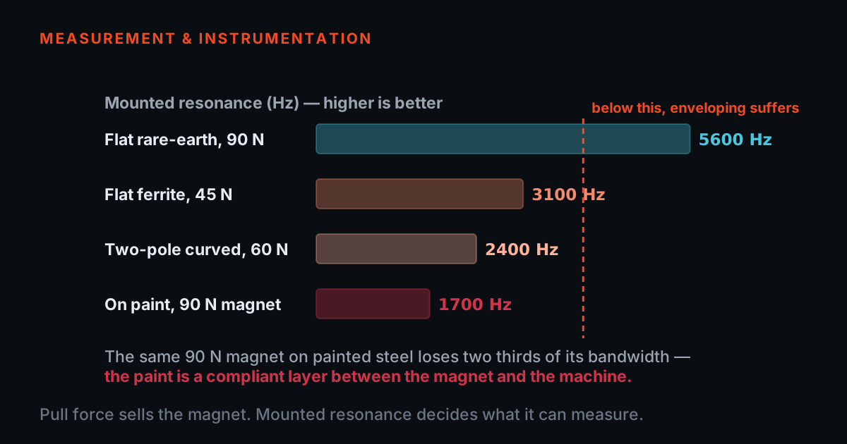
The mounted resonance printed on a datasheet is measured on a stud, into a prepared, flat, clean spot face, torqued to specification. Change the fixture and you change the number. Our mounting bandwidth simulator puts practical ceilings at roughly 10 kHz for a stud, 5 kHz for a thin hard adhesive bond, 1.4 kHz for a flat magnet on clean bare metal and 500 Hz for a handheld probe. Read those against the 2–20 kHz band this whole post is about.
It is worth being precise about how a magnet fails, because the naive version of the warning is wrong and the gate simulator will show you so. A flat magnet resonates around 4.2 kHz. Below that it does not attenuate at all — it amplifies, by about 9.5 dB at 3.5 kHz. Your comb gets taller and your trend gets louder, and none of it is calibrated: the gain depends on the surface, the film of dirt and exactly where the magnet last landed, so the same bearing measured twice gives two different severities. Above its resonance the magnet collapses properly — roughly −8.5 dB at 8 kHz, −17 dB at 12 kHz, −27 dB at 20 kHz — and there the band really is gone.
So a magnet gives you one of two failures depending on where the housing rings: an inflated number you cannot trend, or no signal at all. Neither is a measurement. The pump had both problems at once — a quartz sensor on a two-pole magnet — which is why eleven months of routes produced eleven months of nothing. The argument is made at length in why cheap cables and magnets cost more.
The brochure is specific about the fixture and it is worth honouring. The 621 uses a 5-44 male thread at 2.0 to 2.2 N·m. The 622, 623, 624, 625, 626, 627 and 628 all use ¼-28 at 2.7 to 6.8 N·m, with an M6×1 metric-mount variant available across the range. Every one is welded hermetic, IP68 and rated −54 to +121 °C, with an HT prefix taking the 622, 623, 624, 625 and 628 to +163 °C and an EX prefix certifying the 621, 622, 623, 625 and 628 for ATEX, CSA and IECEx hazardous areas.
The last link is the cable that carries a signal measured in tens of µg through an electrically filthy plant. A low-noise coaxial cable is not an accessory for that job; a triboelectric-noisy one contributes more than the 622's entire noise budget. That argument is made in how vibration cables are tested, and the recording end of it in what makes a DAQ trustworthy.
Act IV · What the plant does now
The pump was rebuilt with a 623C01 stud-mounted into a spot face machined onto the bearing housing, on 12 m of low-noise coaxial cable into a 10 mA conditioner. Bias voltage is recorded at the start of every route as a single line in the sheet. Nothing about the analysis changed; the analyst was never the problem.
The habit worth breaking is buying an accelerometer on sensitivity. 100 mV/g tells you almost nothing about whether a bearing fault will be visible, because sensitivity is a scaling factor and detection is a ratio. Seven of the eight models here are 100 mV/g and they differ by fifteen times in what they can actually resolve.
Read the datasheet in this order instead. Mounted resonance — does the sensor reach the ring? Spectral noise density — can it see the ring once it gets there? Measurement range — will the record survive the machine? Three numbers, in that order, and an eight-model brochure collapses into a shortlist in about a minute.
Then check the fixture, because none of it survives a magnet. And check the loop, because none of it survives 100 m of cable at 4 mA.
The uncomfortable part of this case is that nothing in it was exotic. A correct sensor, specified for the wrong job, on a convenient mount, at the end of a long cable. Every one of those decisions was made by someone reasonable, and none of them was made by the person who later got asked why the bearing failed.
- Read the datasheet in this order: mounted resonance, then spectral noise density, then measurement range
- Stud-mount into a prepared spot face when the housing rings above a magnet's ceiling
- Record the bias voltage at the start of every route, as one line on the sheet
- Check the conditioner current and the cable length against the band you actually need
- Buy on sensitivity — seven of these eight models are 100 mV/g and differ by fifteen times in what they can resolve
- Ask a unit specified for long-term stability to find an incipient spall
- Trend an amplitude taken through a magnet below its resonance — the gain moves with every remount
- Read a clean route as a clean machine when the detection floor may be sitting above the fault
TIERA instruments that do this work.
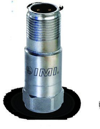
IMI 623C01 — High Frequency ICP® Accelerometer
The default bearing-enveloping sensor, and what the pump runs now: a 40 kHz mounted resonance keeps it flat across the whole ringing band, and 0.9 µg/√Hz keeps the comb above its own noise. Small enough at 17.3 mm diameter and 51 g for crowded pump and motor housings.
- Sensitivity
- 100 mV/g (±5 %)
- Frequency range (±3 dB)
- 0.8 to 15,000 Hz
- Mounted resonance
- 40 kHz
- Spectral noise at 1 kHz
- 0.9 µg/√Hz
- Broadband resolution
- 100 µg (1–10 kHz)
- Mount / weight
- ¼-28 female, 2.7–6.8 N·m / 51 g
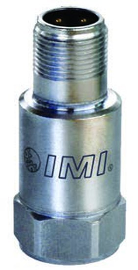
IMI 622B01 — Top Exit ICP® Accelerometer
The lowest noise floor in the precision range — 22 µg across a 3 kHz envelope band, against 329 µg for the quartz units. When the value of the programme is in catching the defect early, this is the sensor that buys the months.
- Sensitivity
- 100 mV/g (±5 %)
- Frequency range (±3 dB)
- 0.2 to 15,000 Hz
- Mounted resonance
- 30 kHz
- Spectral noise at 1 kHz
- 0.4 µg/√Hz
- Broadband resolution
- 50 µg (1–10 kHz)
- Mount / weight
- ¼-28 female, 2.7–6.8 N·m / 94 g
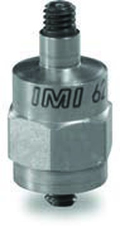
IMI 621C40 — Very High Frequency ICP® Accelerometer
For machines that hammer. ±500 g full scale and a 10,000 g shock limit keep the record unclipped where a ±50 g sensor manufactures the false comb the simulator above computes — and ±3 dB to 30 kHz reaches gear-mesh harmonics nothing else here can see, in 4.75 grams.
- Sensitivity
- 10 mV/g (±10 %)
- Measurement range
- ±500 g
- Frequency range (±3 dB)
- 1.6 to 30,000 Hz
- Mounted resonance
- 85 kHz
- Overload limit (shock)
- 10,000 g pk
- Mount / weight
- 5-44 male, 2.0–2.2 N·m / 4.75 g

PhonoVibe Series — Sound & Vibration DAQ
A sensor that reaches 15 kHz is wasted on a recorder that does not. Q/O/HD sample at 128 kHz across 0.5 Hz – 60 kHz with 24-bit resolution and built-in ICP/IEPE power, so the ringing band survives the whole chain.
- ADC resolution
- 24-bit, simultaneous sampling
- Sampling (Q/O/HD)
- 128 kHz
- Bandwidth (Q/O/HD)
- 0.5 Hz – 60 kHz
- Sensor power
- 24 V, 4 mA (IEPE/ICP/CCLD)
From the TIERA store
The kit for this job
What we would actually put in front of someone doing the measurement this post describes — not the whole catalogue.
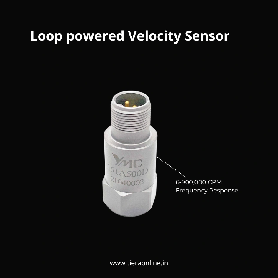 151A500D, 500mV/g Industrial AccelerometerLOW FREQUENCY ACCELEROMETER, TOP EXIT 2 PIN CONNECTOR, 500 MV/G, ±10% 6-600,000 CPM Frequency Response (±3dB) -54 to 121 °C Temperature Range Hermetic Sealing Case isolated₹24,522View →
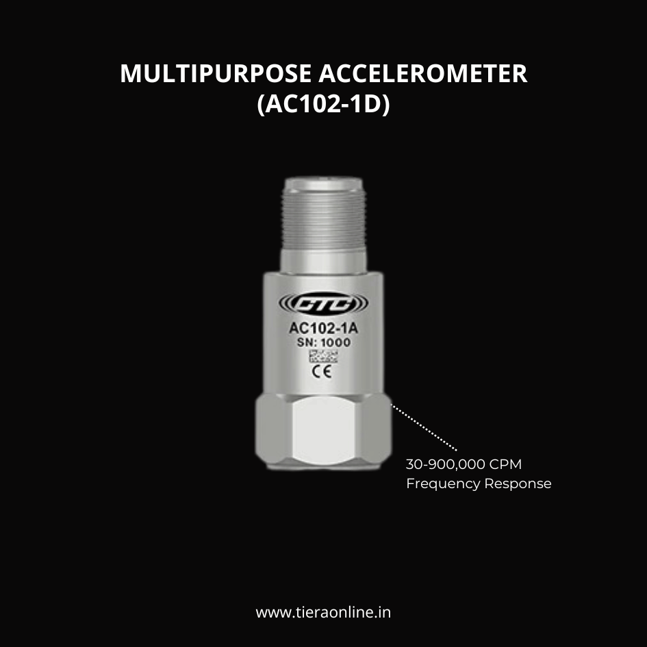 AC102-1D, MULTIPURPOSE ACCELEROMETERMULTIPURPOSE ACCELEROMETER, TOP EXIT 2 PIN CONNECTOR, 100 MV/G, ±10% 30-900,000 CPM Frequency Response (±3dB) -58 to 250 °F (-50 to 121 °C) Temperature Range Welded, Hermetic Sealing CTC’s Best Selling, Multi-Purpose Sensor Ideally Suited for Thousands of Applications₹14,750View →
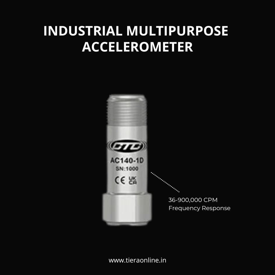 AC140-1D LOW COST MINIATURE INDUSTRIAL MULTIPURPOSE ACCELEROMETERMini Industrial Accelerometer, Great for Hard-to-Reach Locations₹15,000View →
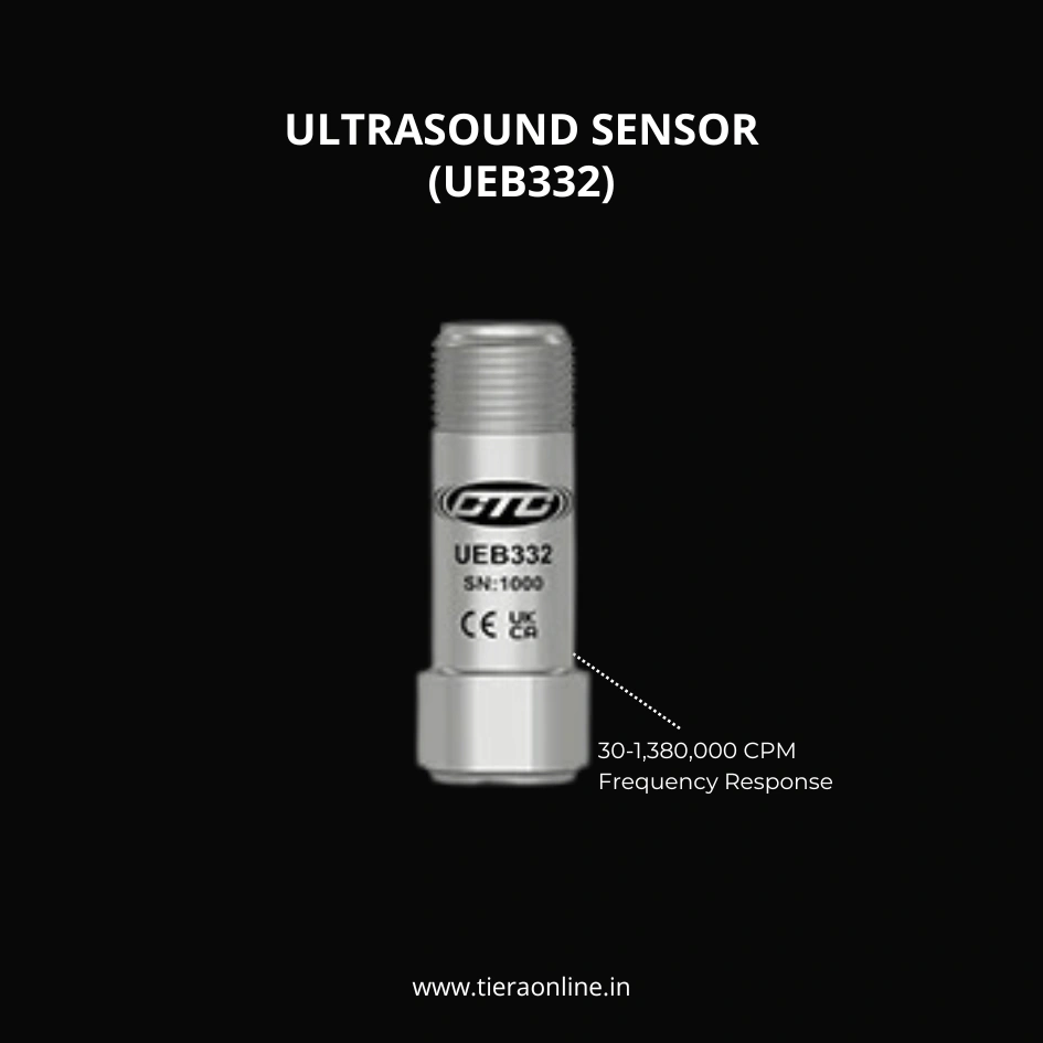 UEB332, ULTRASOUND SENSORCTC’s High Frequency Ultrasound Accelerometer. High Amplitude Resonance Peak for Stress Wave Measurement Techniques. It works on the IEPE Amplifier Technology.₹44,560View →
Use cases
Where this shows up in the field
Tell us the machine — we will tell you which of the eight, and why
TIERA specifies and supplies the IMI Sensors precision ICP range alongside our own PhonoVibe DAQ, TVIB analysis software, and the mounting and cabling that decide whether any of it works. The gates in this post are exactly how we make the recommendation: what the housing rings at, how faint the defect will be when you first want to catch it, how hard the machine hits, and what the cable run and conditioner will actually carry. Give us the machine list — speeds, bearing part numbers, duty, cable runs — and the shortlist usually comes down to one or two models per measurement point.
The models are also available with the prefixes the plant may need: EX for ATEX, CSA and IECEx hazardous areas on the 621, 622, 623, 625 and 628; HT to raise the operating range from +121 °C to +163 °C on the 622, 623, 624, 625 and 628; M for M6×1 metric mounting across the whole range; TO for a built-in temperature output; and VO for a velocity output at 100 mV/ips. Alternate sensitivities of 10, 50 and 500 mV/g are available on most models, and every series offers integral polyurethane or armoured-polyurethane cable versions with configurable length and terminating connector.
And if you want the pattern recognition before the plant provides you with real failures, the TMFSS simulator seeds outer-race, inner-race, cage and rolling-element defects under controlled speed — so the comb in these simulators is one you have already measured with your own hands, through your own sensor, at a severity you chose.
- IMI precision ICP accelerometers, 621 to 628 — specified against your machines, with EX / HT / metric / temperature-output / velocity-output variants
- PhonoVibe Q / O / HD: 24-bit, 128 kHz sampling, 0.5 Hz – 60 kHz, ICP sensor power on every channel — the recording end of the same bandwidth argument
- TVIB TSAP201 (free with every PhonoVibe): FIR/IIR band-pass, FFT to 102,400 points, harmonic and sideband cursors for laying a ruler over the comb
- Stud-mount blocks, adhesive pads and low-noise coaxial cable — the two gates no datasheet protects you from
- TMFSS benchtop fault simulator with seeded bearing defects, for practising the whole chain before it matters
Where this sits on the TIERA learning ladder.
The theory behind this article is covered free, in full, by the TIERA 101 primers: Accelerometer & DAQ Selection 101, Bearing & Gear Analysis 101. They are self-paced, interactive, and end in an exam and a certificate.
TCAT Cat I-IV adds structured analyst training with proctored examinations at exams.tieraonline.in — the free 101 primers cover the theory, TCAT certifies you can apply it.
TIERA 101 is a free introductory primer, not an accredited ISO certification, and its hours do not count towards the formal training ISO 18436 requires.