

The Periodic Table of Machinery Faults — All 67, Column by Column
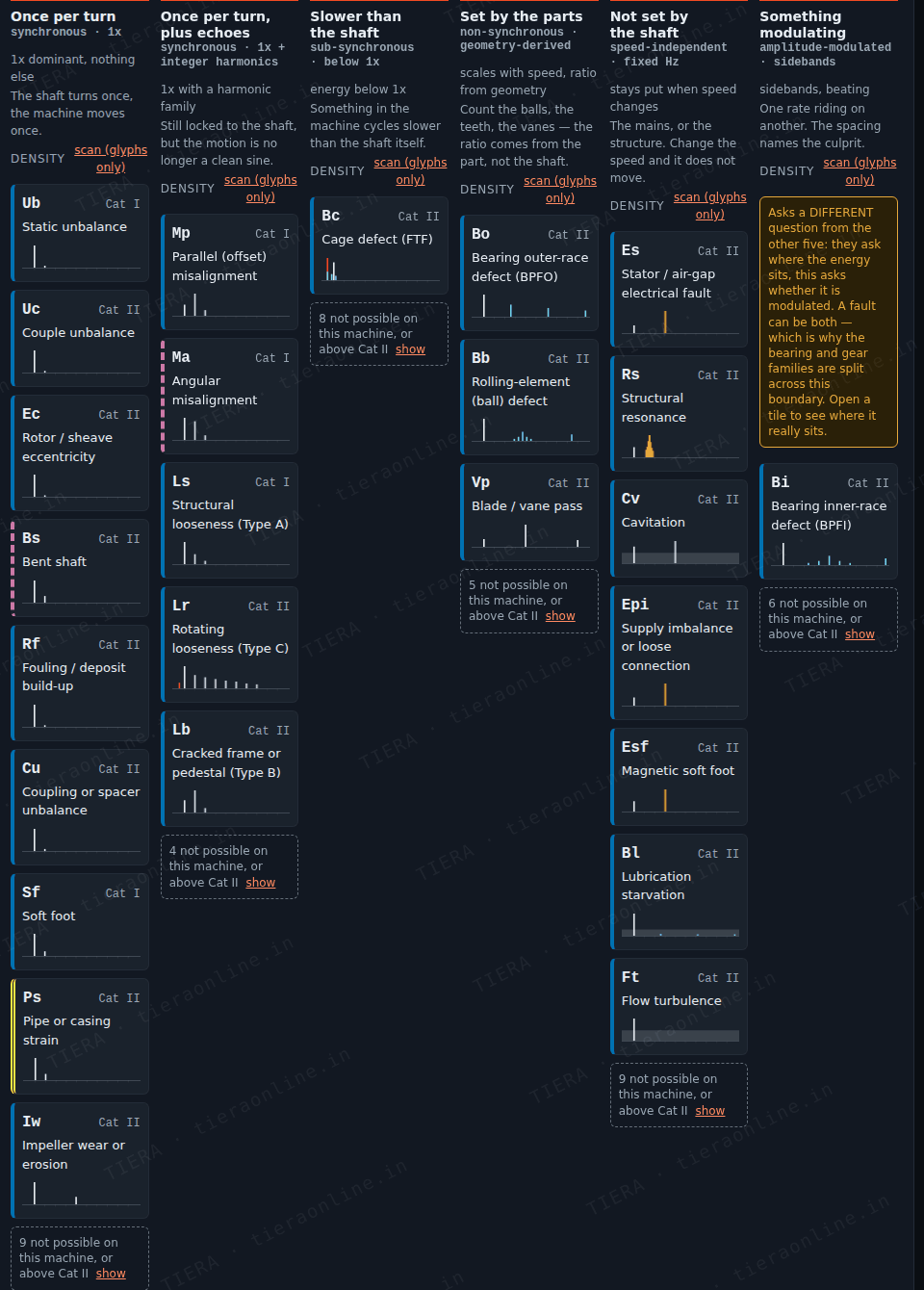
Sort every vibration fault by what its spectrum looks like and you get a recognition index a beginner can enter knowing nothing else. This walks all six columns and names all 67 faults — then covers what the arrangement cannot do: decide, rank your next measurement, or notice that your record was never readable.
Two ways to organise a fault
There are only two honest ways to arrange the faults a rotating machine can have. You can sort them by what causes them — unbalance here, misalignment there, bearings in their own chapter — which is how almost every textbook is written. Or you can sort them by what they look like in a spectrum, which is how a working analyst actually meets them.
The second arrangement matches the order in which you get information. You do not arrive at a machine already knowing it has a cracked pedestal. You arrive holding a spectrum, and something in it caught your eye. The question is not “what does looseness look like?” It is the reverse: “I am looking at this — what could produce it?”
This piece walks the arrangement one column at a time, and names every one of the 67 faults in it. The set is graded by category: 7 at Cat I, 33 at Cat II, 24 at Cat III and 3 at Cat IV — so a beginner can see the shape of what they do not know yet, rather than being shown only the part they are ready for.
The second axis nobody notices: direction
A column tells you where the energy sits in frequency. That is one axis, and on its own it leaves most of the useful information on the table. The second axis is direction — how the same fault divides its energy between horizontal, vertical and axial.
Direction is what separates faults that share a column. Static unbalance and a bent shaft both dominate at 1×, so frequency content cannot tell them apart. Their direction signatures are nothing alike: unbalance is overwhelmingly radial, and a bent shaft puts a large component axially. One extra measurement, taken in a direction you were probably not standing in, resolves a pair that the spectrum alone never will.
Each fault carries its own direction glyph, normalised to its strongest direction, so the shape carries the meaning rather than the colour. That matters for the roughly one in twelve men with a colour-vision deficiency, and it matters for anyone reading a printed report in greyscale.
Column 1 — Once per turn (18 faults)
The question: The shaft turns once, the machine moves once. One tall line at 1×, and nothing of consequence above it.
This is the column beginners reach for first and the one that resolves least, because it is the largest. A tall 1× is not a diagnosis — it is the beginning of one. Eighteen distinct faults produce it, spanning unbalance in four different forms, a bent shaft, a soft foot, pipe strain, fouling, a failed isolator, thermal bow, and two separate resonance conditions.
What separates them is never the height of the 1×. It is direction, phase across the coupling, how the amplitude responds to speed, and whether it changed after the machine was last touched. Anyone who stops at “tall 1× equals unbalance” will balance a machine that was never unbalanced — repeatedly, because the vibration always comes back.
Column 2 — Once per turn, plus echoes (9 faults)
The question: Still locked to the shaft, but the motion is no longer a clean sine. A harmonic family — 1×, 2×, 3× and upward — means the shaft turns once and the machine does something more complicated than move once.
The classic residents are misalignment and looseness, and the pattern of the harmonics separates them better than their presence does. Misalignment tends to put strong energy at 2×, often with a substantial axial component. Looseness spreads energy much further up the series — a picket fence that keeps going — and as it worsens it starts producing half-orders, which is a genuinely different signature rather than a louder version of the same one.
This column also contains the faults that are really joints rather than rotors: a cracked pedestal, grout loss, a worn coupling element, a gear coupling that has locked up. All of them are structures that have stopped behaving as one rigid piece, and all of them announce it by turning a clean once-per-turn motion into something with corners.
Column 3 — Slower than the shaft (9 faults)
The question: Something in the machine cycles slower than the shaft itself. Energy below 1× means something in the machine is cycling slower than the shaft that drives it.
Sub-synchronous energy is rare enough to be a strong clue and serious enough to be worth acting on. A bearing cage turns at roughly 0.4× shaft speed, so cage-rate energy is a bearing telling you it is in trouble. Oil whirl sits near 0.42–0.48× and is a journal bearing losing its film stability; oil whip is what whirl becomes when it locks onto a critical speed, and it is a Cat IV problem that can destroy a machine.
A belt runs slower than either sheave, so belt-rate energy and belt resonance both land here. And a rub — a rotor touching something it should not — generates sub-synchronous energy through an entirely different mechanism, which is why it belongs in this column despite having nothing else in common with the others.
Column 4 — Set by the parts (8 faults)
The question: Count the balls, the teeth, the vanes — the ratio comes from the part, not the shaft. These frequencies scale with speed, but the ratio comes from the geometry of a component rather than from the shaft.
This is the column with the strongest single tell: the peaks do not land on whole orders. A bearing outer-race defect on a typical bearing might sit at 3.58×, with harmonics at 7.16× and 10.74× — a comb that visibly falls between the gridlines. Count the balls and you can predict it; measure it and you can confirm which element is damaged.
Blade and vane pass belong here for the same reason — count the vanes, multiply by shaft speed — and so does gear misalignment, backlash, and the vane-to-cutwater gap problem that produces pressure pulsation in a pump. The convention this registry uses for ball defects is an impact rate of 2×BSF, which is the mainstream reading and worth stating because the alternative convention halves every number you compute.
Column 5 — Not set by the shaft (16 faults)
The question: The mains, or the structure. Change the speed and it does not move. If the peak stays exactly where it is when the running speed changes, it does not belong to the rotor at all.
Two families dominate. Electrical faults are tied to the supply — a stator or air-gap problem, supply imbalance, loose stator laminations, magnetic soft foot, and VFD carrier lines — so they land at mains-related frequencies that a mechanical change cannot move. Structural resonances sit at the natural frequency of the structure, which is a property of mass and stiffness, not of speed.
A resonance has a width, and that width is diagnostic. An electrical line at 100 Hz is a discrete line; a structural mode at 62 Hz has a skirt whose breadth is set by damping, and the half-power method turns that skirt into a damping measurement. A page that drew both as identical single lines would erase the only visual cue separating them.
This column also carries the flow faults — cavitation, recirculation, turbulence, compressor surge, aerodynamic stall — which are broadband rather than tonal, and which announce themselves by raising the floor rather than by adding a line.
The obvious test for this column is to change the running speed and see what moves. Most industrial machines cannot do that. A direct-on-line motor runs at one speed and will not be asked to run 10% faster to satisfy an analyst. So every fault here also carries a route that needs no speed change — otherwise the column would be unreachable on the majority of real assets.
Column 6 — Something modulating (7 faults)
The question: One rate riding on another. The spacing names the culprit.
This column asks a genuinely different question from the other five. They ask where the energy sits; this one asks whether the energy is being modulated. Asks a DIFFERENT question from the other five: they ask where the energy sits, this asks whether it is modulated. A fault can be both — which is why the bearing and gear families are split across this boundary. Open a tile to see where it really sits.
The mechanism is the same in every case: something passes through a varying load or a varying gap, once per revolution of something else. An inner-race defect moves in and out of the load zone as the shaft turns, so its impacts are amplitude-modulated at shaft rate and the spectrum grows sidebands spaced at 1×. A cracked gear tooth does the same at gear-shaft rate. A broken rotor bar modulates at twice slip frequency.
That is why the sideband spacing is the diagnosis and the carrier is only the location. Read the spacing and it names the modulating rate; the modulating rate names the component.
One fault is not one picture — the stage model
A fixed grid has to put each fault in one cell, and that is a real limitation, because many faults migrate as they develop. The registry handles this by treating a fault as a path rather than a point: every fault carries four stages, and each stage synthesises a different signal.
An early rolling-element defect is a clean comb at the race frequency with almost no floor. A developing one grows harmonics. An advanced one adds sidebands as the defect starts passing through the load zone. A terminal one raises the broadband floor so far that it swallows its own comb — the diagnostic feature disappears not because the machine improved but because the damage stopped being discrete.
This is the single most dangerous thing about trending a bearing on overall level: the terminal stage can read as a plateau on the feature you were watching, right before failure.
Before any of it: is the record even readable?
Every fault above is a fault of the machine. There is a second, entirely separate family — faults of the measurement — and the important design decision is that they are not allowed to compete in the same list.
A clipped record is not a hypothesis alongside unbalance. It is a reason the question cannot be answered yet. So the measurement-chain checks form a gate: nothing downstream — no ranking, no belief, no verdict — is offered until the record is known to be readable.
The gate checks for clipping and input overload, a settling ramp or dropouts, a dead or desensitised sensor, cable break and intermittent connection, DC settling and ski-slope, ground loops and line-frequency pickup, coarse quantisation, external shock during the record, aliasing, and whether the mounting can even reach the bandwidth the suspected fault needs. A magnet-mounted sensor cannot deliver a 5 kHz bearing band, and no amount of analysis recovers what the mount rolled off.
This matters more than another dozen machine faults would. In real fleets, bad records are far more common than exotic faults — and a table that reads a bad record will route you confidently into the wrong column.
What to measure next — ranked by bits per minute
A layout hands you a shortlist and stops. The question an analyst actually faces next is different: what should I measure now, and is it worth the walk?
That question has a real answer. Treat the candidates as a probability distribution, and each candidate measurement has an expected information gain — how much it should reduce your uncertainty, in bits. Divide that by what the measurement costs in minutes, and you get a ranking of what to do next.
The ranking by bits per minute is frequently not the ranking by bits. A measurement that would resolve more of the uncertainty but takes four times as long loses to a cheaper one that resolves less. And a measurement requiring a shutdown carries an explicit penalty, because stopping a machine is not a scheduling inconvenience — it is often the most expensive thing in the whole diagnosis.
Two things have to be said plainly about this. The likelihoods behind it are elicited from engineering judgement, not measured from field statistics — so the arithmetic is exact and its inputs are opinions, and every number it produces should be read that way. And the prior is uniform: it does not know that your plant replaces couplings badly, or that this machine has been balanced three times this year.
Where two faults genuinely cannot be separated
The most instructive thing about laying faults out this way is what happens at the edges — and the honest version of that requires measuring it rather than asserting it.
Every fault in the registry synthesises a real signal, so the scalar features a condition-monitoring classifier would consume can be computed. That turns “these two are confusable” from a hand-written opinion into a distance in a measured feature space, and the two are then checked against each other. Where the hand-authored list and the computed distance disagree, the disagreement is shown rather than quietly resolved — because a hand-authored list can be incomplete, and a feature bank that cannot see phase will call two faults close when a phase reading separates them instantly.
Some collisions are genuine physics. Two peaks less than one resolution bin apart are not “hard to tell apart”; they are not present as two peaks in that record, and no interpretation recovers what the measurement never captured. A longer record or a different measurement is the only route.
Others are collisions of the layout: faults a spectrum-shape sort files together that direction, phase or a load change separates immediately. Knowing which kind you are looking at is most of what separates a Cat II analyst from a Cat I one.
Speed, and why a slow machine is a different job
Everything above quietly assumes a machine turning fast enough for a spectrum to mean something. Below a few hundred rpm that assumption fails, and it fails in four independent ways at once — which is why “just take a longer record” is not the whole answer.
Energy. For a given displacement, acceleration scales with frequency squared. A defect at 30 rpm produces a tiny fraction of the acceleration the same defect produces at 1490 rpm, and it can sit below the sensor's own noise floor.
Resolution. Frequency resolution is the reciprocal of record length. Separating a cage rate from a shaft rate on a slow machine needs a record measured in minutes, not seconds.
Sensor low-frequency limit. Standard accelerometers roll off at the bottom of their range, so the very frequencies of interest are the ones being attenuated by the instrument.
Bearing impacts stop being impulsive. Enveloping relies on a defect exciting a high-frequency resonance. At low speed the energy may not be enough to ring it, and the technique quietly stops working rather than obviously failing.
A low-speed bearing is therefore a different job with different instruments, not a harder version of the same one — and a table that ignored speed would let a learner walk into it unaware.
The machine is a drivetrain, not a pair
The commonest awkward asset on a real route is not a motor and a pump. It is a motor driving a belt into a gearbox driving a fan — three shafts at three different speeds, in one asset, with one route sheet.
A model that describes a machine as one driver and one driven cannot express that, and it fails in the worst possible way: it looks like it works. You can set “belt” and “gearbox” at the same time and nothing anywhere says whether the belt is before or after the gearbox, or that they turn at different speeds. Every order you then compute is referenced to a shaft that may not be the one you measured.
So the model is a drivetrain: an ordered chain of elements, each with its own speed ratio, and every measurement point tied to the shaft it actually sits on. Orders are then referenced to that shaft, and energy transmitted from neighbouring shafts is computed and listed rather than silently folded into the same waveform.
Health, prognosis, and two refusals worth copying
A health index is a construct, not a measurement — and a single number is exactly the shape of thing that gets trusted without being checked. So it never travels alone: monotonicity (does it move one way as damage accumulates?) and trendability (is it correlated with time at all?) are the two statistics that say whether the index is worth plotting, and they belong beside it every time.
A projection is more dangerous still. It is the number a planner acts on, it looks like a measurement, and nothing in “RUL 47 days” admits it was fitted to four points. Two refusals are therefore built in.
A non-positive slope has no crossing. If the fitted line is flat or falling, the honest return is “no projection”. The algebra would happily produce a number — a large negative one, or a date in the past — and that number would be nonsense presented as arithmetic.
A projection is a band, never a point. The output is a prediction interval, because the interval is the part that is true. A single date is a claim no condition-monitoring model can support.
And the plateau is the trap. Many degradation paths run down, flatten for a long stretch as surfaces work-harden or debris redistributes, then accelerate. A straight-line fit through the plateau projects a comfortable remaining life shortly before failure — which is precisely the wrong answer at precisely the wrong moment.
Exporting it as a labelled dataset — and the split that decides everything
Because every fault synthesises a real signal and every signal yields a computed feature vector, the whole registry can be swept — fault × stage × speed × seed — and emitted as labelled rows a classifier or an RUL model can consume.
One rule governs whether that dataset is worth anything: groups are physical assets. Every row carries the asset it came from, and any split has to keep an asset entirely on one side. Split by row and a model memorises the machine — same mounting, same background, same resonances — then scores brilliantly on more rows from that same machine and collapses on the next one.
Splitting by run or by file is not enough either, for the same reason: two runs on one machine still share everything that makes memorisation possible. The unit of independence is the asset.
The other two rules that get broken: every transform is fitted on training data only, and every score is reported beside its majority-class baseline. A 70% accuracy against a 68% baseline is a result worth almost nothing, and it is reported as 70% far more often than it should be.
What the arrangement is good at, and what it will never do
It is a recognition index, and at that one job it is excellent. It narrows the field fast, and a beginner can enter it knowing only what the spectrum looks like. It also makes the look-alikes visible, which a fault-by-fault chapter list never does.
It cannot decide. A shortlist is not a diagnosis, and nothing in a layout says which candidate is more likely on this machine, on this day, given what you measured last month.
It cannot rank your next measurement. A grid holds positions, not probabilities, so it cannot weigh a four-minute phase reading against a twenty-minute trend review. That needs an engine, and the engine needs to say out loud that its likelihoods are elicited.
It cannot express a fault that changes with severity. One cell, one appearance — and the stage model exists precisely because that is not how faults behave.
A misleading appearance misleads it completely. Its entire input is what the spectrum looks like. If the record is untrustworthy, it will route you confidently into the wrong column, which is why the measurement-chain gate has to run first.
Use it for the first ninety seconds in front of an unfamiliar spectrum. Stop using it the moment you have a shortlist — from there the work is evidence, not recognition.
Attribution: a periodic-table arrangement of vibration faults was introduced by Dan Ambre, P.E. (Uptime, 2012). TIERA's fault set, symbols, column labels, direction axis and colour system are our own.
TIERA instruments that do this work.

TMFSS — Machinery Fault Signature Simulator
Produce each column's signature on a real machine, on demand, and watch the look-alikes collide for yourself.
- Fault library
- 30+ faults in the base kit
- Expandable
- Gear, belt, resonance and cavitation kits
- Use
- Training, validation, AI dataset generation

TVIB — Sound & Vibration Analysis Software
Phase and direction — the second axis the table cannot give you, and the one that settles most collisions.
- Analysis
- Time, FFT, FRF, octave, order tracking
- Diagnostics
- Phase, balancing, spectral alarms

PhonoVibe Series — Sound & Vibration DAQ
The measurement chain the whole method rests on — because a misleading record routes you into the wrong column.
- Channels
- 2, 4, 8 and 16
- Resolution
- 24-bit
From the TIERA store
The kit for this job
What we would actually put in front of someone doing the measurement this post describes — not the whole catalogue.
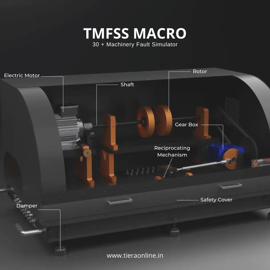 Machinery Fault Signature SimulatorTiera’s Machine Fault Simulator (TMFSS) is a valuable tool for industries and researchers, simulating over 30 real-world faults such as: Bearing faults: outer race defects, inner race defects, cage defects. Motor faults: stator faults, rotor faults, electrical unbalance. Gearbox faults: gear wear, misalignment, gear tooth damage. Etc..₹13,53,600View →
- Machinery Fault Signature Simulator | TMFSS MINIThe TMFSS Mini is Tiera’s compact yet powerful machinery fault simulator designed to provide hands-on learning and experimentation in fault diagnosis and vibration analysis. Ideal for educational institutions, research labs, and professionals, the TMFSS Mini enables users to simulate real-world machinery faults in a controlled environment.Request priceView →
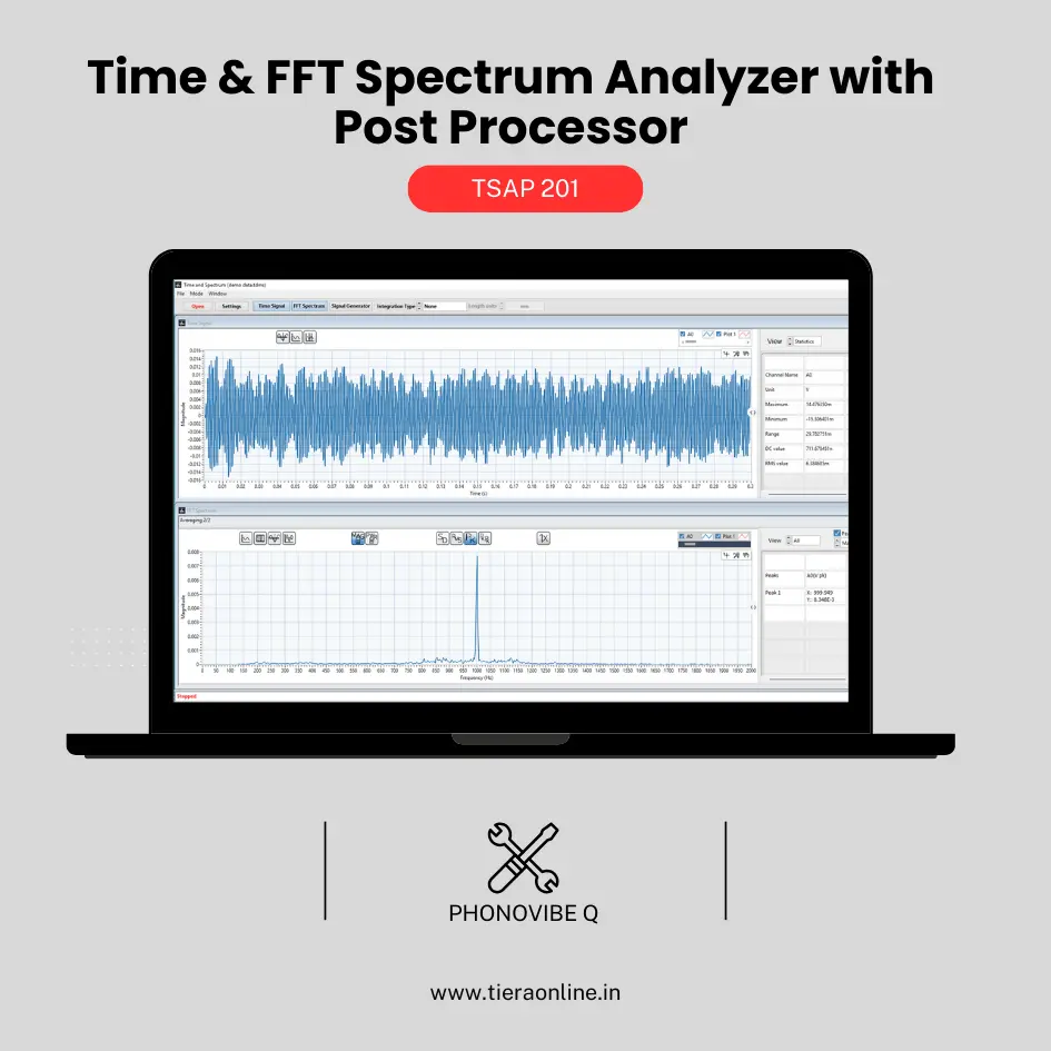 TSAP 201 -Time & FFT Spectrum Analyzer with Post Processor (Phonovibe Q)Use Cases Bump Test Product Development Off route Machine Vibration analysis. Drop Test Product Development & Research₹34,560View →
- Training KitsCompact, classroom-friendly hardware bundles that pair with TCAT Cat I / Cat II syllabi — bearing-fault rigs, balancing benches, and structural-modal demonstrators. Designed to fit a 6-ft table.Request priceView →
Use cases
Where this shows up in the field
Learn the shortlist, then learn what settles it.
A recognition index gets a new analyst moving on day one. What turns that into a diagnosis is a machine you can put a known fault into, and an analyser that shows you the axis the table does not have.
TMFSS lets a trainee produce a fault deliberately, look at it, then produce its nearest look-alike and fail to tell them apart — which is the lesson that sticks.
- TMFSS Macro and Mini — seeded faults across every column in the table
- TVIB — phase and direction, the second axis that separates the collisions
- TCAT Cat I and Cat II — where the judgement half is actually taught
Where this sits on the TIERA learning ladder.
The theory behind this article is covered free, in full, by the TIERA 101 primers: Machinery Fault Diagnosis 101, Bearing & Gear Analysis 101. They are self-paced, interactive, and end in an exam and a certificate.
The free primer covers reading the columns. Deciding between the tiles in one column — ranking the next measurement, weighing evidence, knowing which collisions are physics and which are the layout's — is the Cat II material.
TIERA 101 is a free introductory primer, not an accredited ISO certification, and its hours do not count towards the formal training ISO 18436 requires.