Is It the FFT's Problem or the Machine's? The Peak That Moves When You Change a Setting
Half of what analysts call a fault is the transform talking. This post gives every artifact a test you can run in sixty seconds: change one acquisition setting and see whether the peak moves. Two live simulators, every number computed rather than quoted — including three results that contradict the usual telling.
Two analysts, one spectrum, opposite verdicts
A spectrum arrives with a tidy pair of lines either side of 1x. One analyst calls modulation and books a gearbox inspection. The other changes the record length, watches the spacing between those lines change from 1.00 Hz to 2.00 Hz to 4.00 Hz, and calls it leakage. Both were looking at the same machine. Only one was looking at the machine.
The FFT is not lying to you. It is answering a question you may not have realised you asked: given this many samples, taken at this rate, over this length of time, multiplied by this window — what sinusoids would reproduce that record exactly? Every setting in that sentence is yours. Change one and the answer changes, and the change has nothing to do with the steel.
That gives us the one rule this entire post runs on, and it is testable rather than philosophical: an artifact responds to a setting change; a fault does not. Everything below is that rule, applied to one phenomenon at a time, with the arithmetic done rather than asserted.
Three of the results contradict how this is usually taught. A constant DC offset does not raise your spectrum — a drift does, and they need different fixes. Leakage buries sidebands far more often than it fakes them. And smearing never manufactures a 0.5x line, whatever you may have read; it manufactures a hump. Each of those is a computation you can repeat, and each is below.
The bench: change one setting, watch what moves
Read the rest of this post with this open. The machine preset is fixed — it genuinely does not change while you drive the acquisition settings, which is the whole point. Pick a machine, press Hold as reference, then change exactly one thing and read the verdict.
The verdict is computed, not looked up. It compares the live peak against the reference you held, allows a real line up to half a bin of scalloping shift and up to 4.5 dB of window-dependent amplitude change, and only then decides. If you change the machine preset it will tell you that is not a fair test, because it is not.
The maths underneath is honest. The signal is synthesised at eight times the sample rate, hard-clipped at whatever input range you chose, and then decimated with no anti-alias filter at all — so when something aliases, it aliases for the real reason. The spectrum is a radix-2 FFT with coherent-gain correction, so a tone sitting on a bin reads its true amplitude; the fainter continuous curve is the same record transformed with four times zero padding, which is what actually lives between the analyser's bins.
Δf = 1/T, and why zero-padding is a lie of omission
- Zero-padding interpolates. It reads a peak's position more precisely and is completely powerless to separate two features the record was too short to separate.
- Sixty-four times padding on a half-second record produced 16,384 numbers and still one peak; a four-second record split the same two lines cleanly with no padding at all.
- The test: double the record length. Real close lines split, an interpolated curve just gets smoother.
Resolution is not a setting. It is a consequence: Δf = 1/T. Choose 400 lines and an Fmax and you have chosen a record length, and that record length is the only thing that decides whether two close features are two features or one. Our sample-rate explainer at /blog/sample-rate-fmax-antialias works through the Fmax, lines and capture-time arithmetic properly; this post cares about one consequence of it.
Take two genuine lines 3 Hz apart, at 50.0 and 53.0 Hz, and a half-second record — Δf = 2 Hz. The analyser shows one peak at 52.00 Hz. Now zero-pad. Four times: still one peak. Sixteen times: one peak. Sixty-four times, a 16,384-point transform on 256 real samples: still one peak, at 51.50 Hz. Give it a four-second record instead, with no padding at all, and the two lines appear cleanly at 50.00 and 53.00 Hz.
Zero-padding interpolates. It draws a smoother curve through information you already had, which is genuinely useful for reading a peak's position more precisely, and it is completely powerless to separate things the record was too short to separate. As a rule of thumb two features need to be at least 1/T apart to separate at all, and with a Hann window you want roughly twice that before you would swear to it in a report.
The discrimination test is the simplest in this post. Double the record length. Real close lines split. An interpolated curve just gets smoother.
The peak that marches: buying resolution can destroy the peak you bought it for
- No energy is lost when a line smears — the record's RMS held at 0.7071 g through every measurement. The transform simply spread the same energy over more bins.
- That is why an alarm set on 1x amplitude can go quiet on a machine that is getting worse, and why two analysts on different line counts report different severities and are both reading their instruments correctly.
- The test is to make the record shorter and read consecutive blocks: a drifting line's peak marches monotonically, a genuinely broadband hump's peak jitters at random around its centre.
Here is the result that catches almost everyone, including people who have been reading spectra for twenty years. Longer records give finer bins. Finer bins are better. Therefore longer records are better. That chain of reasoning is wrong whenever the machine will not sit still.
Take a 1x line at 50 Hz, 1.000 g peak, on a machine whose speed is drifting at 0.5 Hz/s — thirty RPM per second, which is an unremarkable load swing. Over a record of length T the line sweeps R·T Hz. The bins are 1/T wide. So the smear, measured in bins, is R·T². Doubling the record does not double the problem. It quadruples it.
The measured consequence: at T = 0.25 s the peak reads 1.0000 g. At 1 s, 0.9981 g. At 2 s, 0.9712 g. At 4 s, 0.6975 g. At 8 s, 0.3532 g — the line has lost 9 dB of height purely because you asked for finer resolution. And the record's RMS across every one of those measurements is 0.7071 g, unchanged to four figures. No energy went anywhere. The transform simply spread it across thirty-two bins instead of concentrating it in one.
This is why an alarm set on 1x amplitude can go quiet on a machine that is getting worse, and why two analysts using different line counts will report different severities on the same bearing and both be reading their instruments correctly.
The discrimination test is not to make the record longer. It is to make it shorter, and then look at consecutive blocks one at a time. A drifting line's peak marches monotonically: 50.1, 50.4, 50.6, 50.9, 51.1, 51.4, 51.6, 51.9 Hz across eight half-second blocks. A genuinely broadband hump's peak jitters at random around its centre: 49.6, 48.3, 49.6, 50.7, 50.1, 49.8, 48.6, 49.9 Hz. Marching means the machine changed speed. Wandering means the machine really is broadband there. One long average can never tell you which, because it has already added them together.
If the machine's speed is genuinely wandering, the cure is not a window or a longer record — it is to resample against a tacho so the spectrum is in orders rather than hertz. That is a whole discipline and it has its own post at /blog/order-tracking-variable-speed.
The left edge: a constant offset and a drift are not the same problem
- A constant offset is periodic in any record, so it leaks nowhere. Under a rectangular window it lands entirely in bin 0; under Hann it becomes one phantom line in the first bin, at the full amplitude of the offset.
- What genuinely raises the whole low end is a trend — sensor drift, thermal settling, IEPE recovery — because a trend is not periodic in the record.
- The test: remove the mean, then remove the trend, then high-pass. If the left edge collapses at any of those three steps, it was never motion.
It is widely taught that a DC offset raises your spectrum. It does not, and the reason is worth ten minutes of anyone's time.
A constant offset is perfectly periodic in any record you care to take — it is the same value in every sample, so it repeats trivially. Nothing to leak. With a rectangular window all of it lands in bin 0. Measured with a 1.0 g offset added to a 0.100 g line at 50 Hz: the levels at 1 Hz, 10 Hz and 30 Hz are 0.000000, 0.0000000 and 0.0000000 g. The offset touched nothing.
Apply a Hann window to that same constant offset, though, and something more interesting happens. A Hann window is 0.5 − 0.5·cos(2πn/N), so its transform is non-zero at exactly two places: bin 0 and bin 1. Your 1.000 g offset therefore produces a 1.000 g line in the first bin — a phantom peak, at 0.25 Hz on a four-second record, with the full amplitude of the offset and no physical existence whatsoever. It is not a raised spectrum. It is one spurious line, and if your Fmin starts at zero you will see it every time.
What genuinely raises the whole low end is a trend: sensor drift, thermal settling after clamping a cold accelerometer to a hot housing, the exponential recovery of an IEPE sensor after power-up. A trend is not periodic in the record, so it leaks, and it leaks in a very particular way. With a rectangular window a 1.0 g/s ramp produces exactly 1/(πf): 0.31831 g at 1 Hz, 0.03184 g at 10 Hz, 0.01063 g at 30 Hz — matching the closed form to five figures. With a Hann window the same ramp gives 0.0000199 g at 10 Hz, sixteen hundred times lower.
And here is the practical sting. Almost every analyser offers “remove DC”. Applied to that trend, removing the mean changes the level at 10 Hz from 0.03184 g to 0.03184 g — that is, not at all. Removing the linear trend takes it to 0.00001 g. Two buttons that sound like the same button, and only one of them does anything. Removing the trend also recovers the 1x itself: the untreated ramp had biased that 0.100 g line down to 0.0937 g, a 6.3% amplitude error on the peak you actually came to measure.
All of this matters far more than it sounds, because integration multiplies it. Dividing by ω twice turns a low-frequency wobble you cannot see in acceleration into hundreds of microns of displacement — at 0.5 Hz, half a milli-g becomes 497 µm peak. That story, and how to integrate without lying, is in /blog/acceleration-velocity-displacement.
The discrimination test: remove the mean, then remove the trend, then high-pass. If the left edge collapses at any of those three steps, it was never motion.
What the window decides: not how tall, but whether you see it at all
- A rectangular window did not mis-measure the 0.010 g line six and a half bins from a large 1x — it deleted it, and reported its own skirt instead. No cursor work, averaging or trending recovers that.
- Next to a full-scale tone with a Hann window, a 24-bit converter's real floor sits 32.9 dB below what the window's skirt lets you observe: at 12 and 16 bits you are looking at the ADC, at 20 and 24 bits you are looking at the window.
- The test: change the window. If a line appears or vanishes, the window was the fault — not the machine, and not the converter.
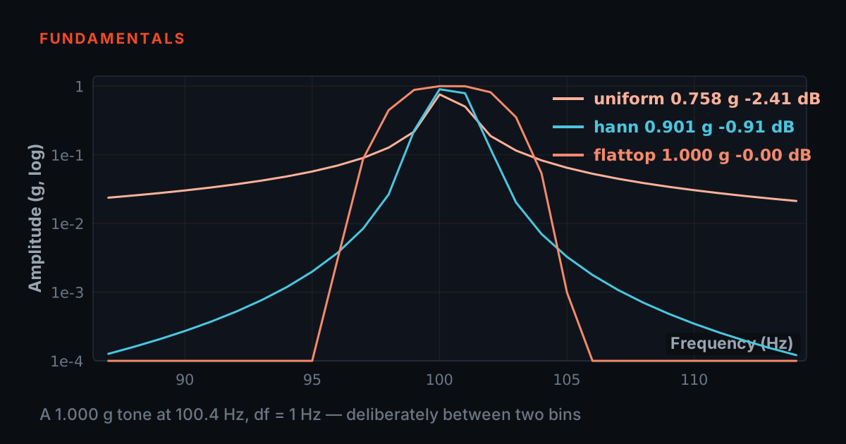
Our window comparator at /blog/fft-window-comparator covers what a window does to amplitude accuracy — rectangular can under-read a peak by 36.2%, Hann by 15.1%, flat-top by 0.1%. Go and drive that one if you have not. This section is about the other thing a window decides, which is rarely taught and matters more for diagnosis: what you can see at all.
Put a 1.000 g line at 50.5 Hz — the worst case, half a bin off centre — and a small 0.010 g line at 57 Hz, forty decibels down and only six and a half bins away. That is a perfectly ordinary situation: a large 1x and a small sideband or bearing tone beside it. With a rectangular window, the big line's leakage skirt at 57 Hz is 0.04611 g, or −26.7 dB. The small line is 0.010 g. It is buried four times over; the analyser reads 0.04040 g there and it is all leakage. With a Hann window the skirt at the same place is 0.00119 g, and the reading becomes 0.01080 g — the small line is plainly there. With flat-top the skirt is 0.00002 g.
So the rectangular window did not merely mis-measure the small tone. It deleted it. No amount of cursor work, averaging or trending recovers a line that the window's own skirt has swallowed.
There is a corollary that is worth knowing before you pay for converter bits. Quantisation noise theory is exact — measured against a dithered 12, 16, 20 and 24-bit converter, the per-bin floor matched q/√12 divided by √((N/2)/ENBW) to within 0.1 dB in every case. But that is the floor the converter has, not the floor you can see. Next to a full-scale tone with a Hann window, a 24-bit converter's real floor of 1.63 nano-g per bin sits 32.9 dB below what the window's leakage skirt lets you observe. At 12 and 16 bits you are looking at the ADC. At 20 and 24 bits you are looking at the window. Buying more bits does not lower the floor you are actually looking at; changing the window does.
The discrimination test: change the window. If a line appears or vanishes, the window was the fault — not the machine, and not the converter.
What the FFT gets right
- The four patterns analysts lean on hardest — broadband impacts, the comb from repeated impacts, harmonics from non-sinusoidal motion, and sidebands from modulation — are all genuinely physical, not artifacts of the transform.
- Real sideband spacing is a property of the machine: 5.00 Hz at record lengths of 1, 2 and 4 seconds. A genuine 0.5x line reads 0.150 g under every window and every record length you try.
- These are the control group. They have no discrimination test because they pass every one.
It would be easy to finish this post believing the spectrum cannot be trusted. The opposite is true: when the acquisition is honest, the FFT renders machine physics with complete fidelity, and the four patterns analysts rely on most are all genuinely physical.
An impact really is broadband. A single 0.5 ms half-sine impact spreads its energy essentially flat from DC upward — measured at −0.0 dB at 100 Hz, −0.5 dB at 500 Hz, −2.1 dB at 1,000 Hz — with the envelope's first null at 2,979 Hz against a theoretical 1.5/τ = 3,000 Hz. That energy is not leakage. It is where the energy physically is, which is exactly why enveloping works and why /blog/bearing-envelope-explained is the next thing to read if bearings are your problem.
Repeated impacts really do comb. Drive the bench above with the impacts preset and read the spectrum: 0.3924 g at 100 Hz, 0.3497 at 200, 0.2862 at 300, 0.2113 at 400 — and exactly 0.0000 at 150, 250, 350, 450 and every other point between. The envelope's null lands precisely on 750 Hz, which is 1.5/τ for the 2 ms impacts. The broad band is the impact; the lines are the rate. Change the record length from 1 s to 2 s to 4 s and every one of those numbers is unchanged to four decimal places.
Harmonics really do come from non-sinusoidal periodic motion. A square wave — the crudest possible model of a machine that slams rather than swings — gives a fundamental of 4/π = 1.2732 and harmonics at exactly −9.54 dB and −13.98 dB, matching 1/3 and 1/5 to two decimals. Nothing was invented by the transform. What each harmonic pattern means for looseness, misalignment and unbalance is the subject of /blog/spectrum-builder-simulator.
Sidebands really do come from modulation. A 50 Hz carrier with 20% amplitude modulation at 5 Hz produces sidebands at 45 and 55 Hz at exactly 0.100 of the carrier — −20.0 dB, which is m/2 to three decimal places. And crucially their spacing is a property of the machine: measured at record lengths of 1, 2 and 4 seconds, the spacing reads 5.00 Hz, 5.00 Hz and 5.00 Hz. Gear sidebands get the full treatment in /blog/gear-mesh-sideband-explorer.
Subharmonics really do come from rub, looseness and oil whirl. A genuine 0.5x line of 0.150 g reads 0.150 g under a rectangular window, 0.150 g under Hann, 0.150 g under flat-top, and 0.150 g at record lengths of 4, 2 and 1 seconds. It does not care what you do to the analyser. That is precisely what makes it real.
These are the control group. They have no discrimination test because they pass every one.
Where the maths imitates the physics
Now the part that costs money. Four cases where the transform produces exactly the pattern a fault would have produced — each with the number that gives it away.
Clipping manufactures harmonics. Feed a pure 1.000 g sine into a ±0.8 g input range and 40.6% of the samples hit the rail. The spectrum then shows a 1x of 0.8959 g, a 3x of 0.0733 g and a 5x of 0.0311 g, on a signal that contains no harmonics at all. Two things give it away. First, the harmonics are strictly odd — 2x reads 0.0000 and 4x reads 0.0000, because symmetric clipping is an odd nonlinearity, and a real looseness or misalignment series is almost never odd-only. Second, and decisively: increase the input range until nothing clips and the harmonics vanish completely. A real 3x does not vanish when you change the gain. Whether your front end is even capable of telling you it clipped is a hardware question, covered in /blog/daq-quality-and-testing.
Leakage fakes a sideband pair — but only in one specific way, and not the way it is usually described. The rectangular window's skirt around an off-bin tone is monotonic on both sides; it is a tent, not a set of discrete lines, and it does not synthesise sidebands. What it does do is split the tone into a doublet. Put a 1x at 50.6 Hz on the bench with a rectangular window and a one-second record: two lines, 0.7550 g at 51.00 Hz and 0.5064 g at 50.00 Hz, one hertz apart. That reads exactly like a sideband pair. Halve the record and they become 50.00 and 52.00 Hz, two hertz apart. Halve it again and they are 52.00 and 48.00, four hertz apart. The spacing is always Δf, because the spacing is Δf. Set the same test against real modulation and the spacing reads 5.00 Hz at every record length you try. Spacing that follows the setting is arithmetic; spacing that follows the machine is a fault.
But leakage's more common crime is the opposite of faking sidebands: it hides them. That is section six, and it is by some distance the more expensive of the two failures, because a fake sideband gets investigated and a hidden one does not.
Beating fakes modulation. Two real lines at 50.0 and 51.3 Hz, 1.000 g each. At T = 0.25 s the analyser shows a single peak whose height swings between 0.218 and 1.693 g from block to block — a 17.8 dB swing on a machine doing nothing unusual. At 0.5 s the swing is 8.7 dB, at 1 s it is 6.0 dB. Take T to 2 s and the peak splits into two steady lines and the swing collapses to 0.3 dB. Nothing about the machine changed between those measurements. The block-to-block amplitude swing is the tell: a peak that will not hold still between consecutive blocks is usually under-resolved, not unstable.
Smearing fakes sub-synchronous energy — as a hump, never as a line. This is the one most often stated wrongly. A 1x drifting at 0.5 Hz/s puts −146.4 dB at 0.5x. That is nothing at all; smearing does not create a discrete subharmonic. What genuinely raises the sub-synchronous region is rectangular-window leakage: an off-bin 1x under a rectangular window reads −48.9 dB at 5 Hz, −48.6 dB at 10 Hz, −46.3 dB at 25 Hz and −44.9 dB at 30 Hz — a broad, almost flat shelf right across the region where you would look for oil whirl. Those absolute levels depend on the record length and on how far off-bin the line happens to sit — the shape does not, and it is the shape that misleads. Switch to Hann and that shelf drops to around −130 dB. So: a raised sub-synchronous floor that collapses when you window properly never existed. A 0.5x line that survives a window change and a record-length change is real, and is worth acting on.
One more, less dramatic but responsible for a lot of wrong numbers: averaging. “Averaging washes out transients” is true, but averaging is at least four different operations and they are nine decibels apart. Put one impact in one of eight blocks and measure the impact band: the single block containing it reads 0.03043 g. A linear magnitude average of the eight reads 0.00380 g — −18.1 dB, exactly 1/8. An RMS or power average reads 0.01076 g — −9.0 dB, exactly 1/√8. Peak hold reads 0.03043 g, unchanged. If a report says “averaged” without saying which, the number in it is uncertain by 9 dB. Coherence and averaging strategy get proper treatment in /blog/coherence-frf-quality.
And time-synchronous averaging deserves its own warning, because it is a feature and a trap wearing the same coat. TSA is designed to delete anything not locked to the shaft. Measured with a shaft at 64 Hz and a non-synchronous tone of 0.300 g at 176.3 Hz: after 4 averages the tone is down to 0.00646 g, after 256 averages to 0.00098 g, matching the Dirichlet-kernel prediction to three significant figures, while random content falls as the familiar 1/√M. That is exactly what you want for a gear. It is exactly what you do not want for a bearing, whose fault frequencies are not integer orders. If you are hunting a bearing and TSA is on, turn it off and re-measure.
One spectrum, two machines — why you still look at the waveform
- The magnitude spectrum throws away phase, so two completely different waveforms can share it exactly — here to within 1.2 × 10⁻¹⁵ g.
- One of those waveforms trips a crest-factor alarm and sends someone to a bearing; the other does not. Same spectrum, same RMS.
- This is not an artifact to test for. It is a permanent property of the tool, and the answer is to keep looking at the time waveform.
There is a limit to what any of this can tell you, and it is structural rather than a matter of settings. The magnitude spectrum throws away phase. Two completely different signals can share it exactly.
Twenty-four harmonics of 10 Hz with 1/k amplitudes. Put every phase at zero and you get a spiky, impulsive waveform: peak 3.7760, RMS 0.8956, crest factor 4.216. Scramble the phases and leave every amplitude untouched and you get a smooth wash: peak 2.0140, the same RMS of 0.8956, crest factor 2.249. The two magnitude spectra differ by 1.2 × 10⁻¹⁵ g, which is to say by nothing.
One of those waveforms would trip an impact or crest-factor alarm and send someone to look at a bearing. The other would not. The spectrum cannot distinguish them, and no window, record length or averaging strategy will help, because the information was discarded before any of those got involved. This is not an artifact to be tested for. It is a permanent property of the tool, and the answer is simply to keep looking at the time waveform — which, on any analyser worth using, is one click away.
The same discipline applies to how amplitudes get quoted. One 1.000 g peak sine is 0.7071 g RMS and 2.000 g peak-to-peak: the two extremes are a factor of 2.828, or 9.0 dB, apart. And there are two different right ways to correct a windowed spectrum — a tone needs the coherent-gain correction, a noise floor needs the ENBW correction, and applying the wrong one puts flat-top out by a factor of 1.585 on the floor while it reads the tone perfectly. Most arguments about whether a machine is in alarm turn out to be arguments about which of these was meant.
The card: change one setting, then decide
None of this requires new equipment or a course. It requires the habit of changing one thing at a time and watching, which takes about sixty seconds per suspicion and settles most of them.
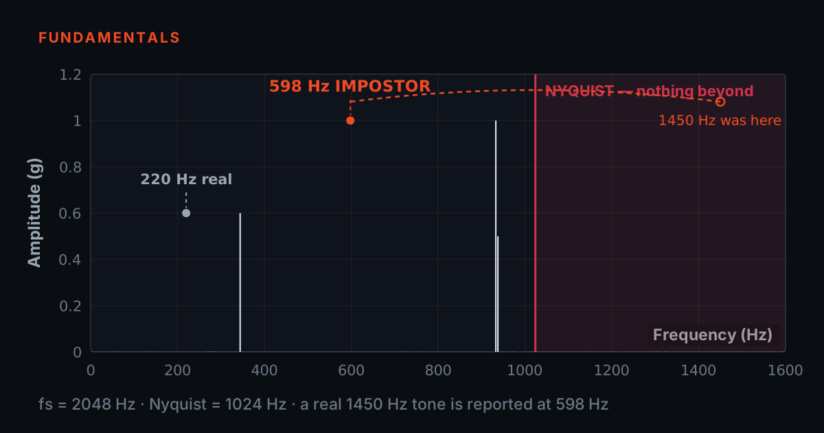
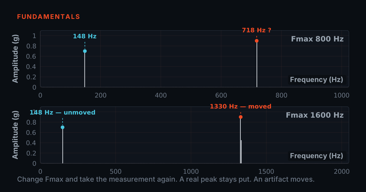
The order matters a little. Start with the window, because it is instant and it separates leakage problems from everything else. Then the record length, which separates resolution problems and exposes beating. Then consecutive short blocks, which is the only test that distinguishes a drifting line from a genuinely broad feature. Then Fmax, which catches aliases. Then the input range, which catches clipping. Then detrending, which catches the left edge. Only then start thinking about the machine.
And when nothing you change moves it — stop adjusting the analyser. You have a measurement, and the measurement is telling you about the machine. Go and look at the machine.
Where to learn this properly
This post is deliberately the connective one. The theory it leans on lives in the posts it points at: windows and coherent gain in /blog/fft-window-comparator, the sampling front end in /blog/sample-rate-fmax-antialias with a live playground at /blog/aliasing-playground-simulator, integration and the ski slope in /blog/acceleration-velocity-displacement, enveloping in /blog/bearing-envelope-explained, and order tracking in /blog/order-tracking-variable-speed. If you want the fault patterns rather than the artifacts, start at /blog/spectrum-builder-simulator.
The underlying theory — the DFT's periodicity assumption, leakage, window figures of merit, resolution and the sampling theorem — is covered free and in full by TIERA's Signal Processing 101 primer, and the front-end half by Accelerometer & DAQ Selection 101, both at 101.tieraonline.in. The primers are free introductory courses for onboarding and refreshing fundamentals, not accredited ISO certifications.
For formal, assessed competence in vibration analysis, TIERA runs the TCAT programme — details on the services page at /services — with proctored examinations at exams.tieraonline.in. A sensible path: the primers first, then an afternoon on a real analyser running the card above against a signal generator, then the formal programme when certification matters.
TIERA instruments that do this work.

TVIB — Sound & Vibration Analysis Software
Every test on the field card is a control you can actually reach: selectable windowing, FFT sizes fine enough to run the resolution test properly, and exponential, linear and peak-hold averaging so you can find the transient the average was hiding.
- FFT size
- Up to 102,400 points
- Averaging
- Exponential, linear, peak hold — selectable windowing
- Cursors
- Harmonic, band and sideband, in time and frequency
- Integration
- Acceleration → velocity → displacement
- Trial
- 14-day fully-unlocked evaluation licence

PhonoVibe Series — Sound & Vibration DAQ
Half the artifacts in this post are front-end problems: 24-bit simultaneous sampling with IEPE power and TEDS means the samples the window multiplies are worth trusting before you start testing them.
- ADC resolution
- 24-bit, across the entire series
- Channels
- 2, 4, 8 or 16
- Sampling
- Simultaneous on every input
- Sensor power
- 24 V, 4 mA (IEPE/ICP/CCLD), TEDS supported
- Software
- TVIB TSAP 201 bundled
From the TIERA store
The kit for this job
What we would actually put in front of someone doing the measurement this post describes — not the whole catalogue.
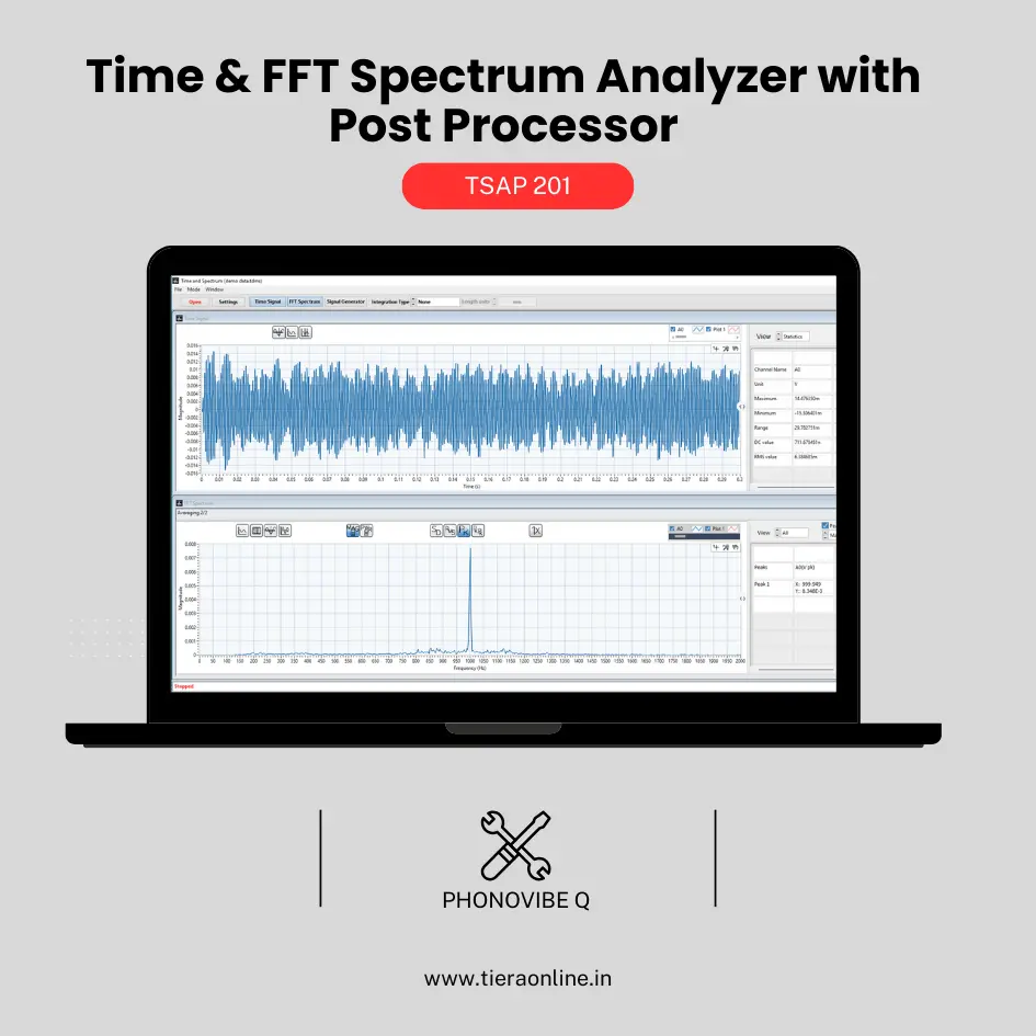 TSAP 201 -Time & FFT Spectrum Analyzer with Post Processor (Phonovibe Q)Use Cases Bump Test Product Development Off route Machine Vibration analysis. Drop Test Product Development & Research₹34,560View →
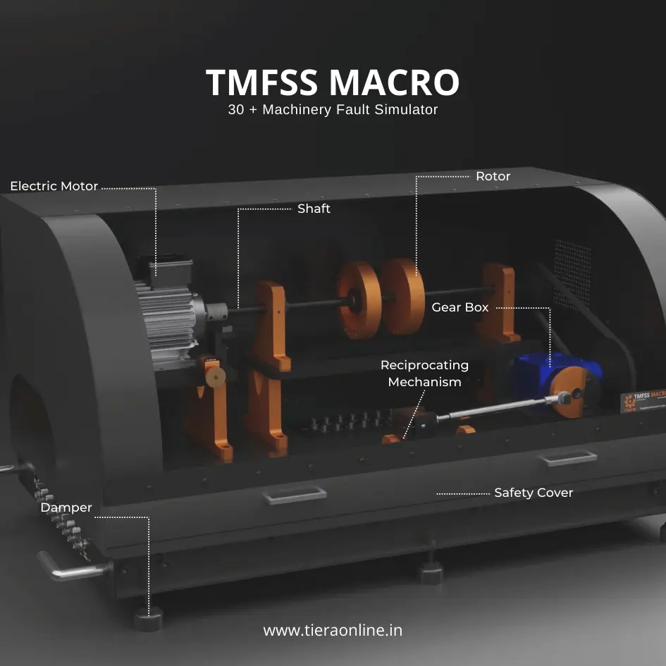 Machinery Fault Signature SimulatorTiera’s Machine Fault Simulator (TMFSS) is a valuable tool for industries and researchers, simulating over 30 real-world faults such as: Bearing faults: outer race defects, inner race defects, cage defects. Motor faults: stator faults, rotor faults, electrical unbalance. Gearbox faults: gear wear, misalignment, gear tooth damage. And more.₹13,53,600View →
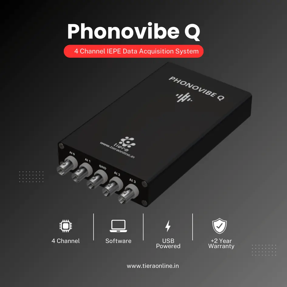 4 Channel IEPE Data Acquisition System – Phonovibe QFour Channels Standard plug & play USB Powered Take data from accelerometers, microphones, hammers, or any other IEPE Sensors T- VIB Software to acquire time waveforms, frequency spectra, overall vibration levels, FRF’s and octave measurements ** Windows 10 or above Operating System ** T-VIB Software base version comes with Time and Spectrum with Post processor TSAP 201. Check out TVIB Software regarding more module options.₹2,88,000View →
Use cases
Where this shows up in the field
An analyser where every test on that card is one click away
The whole method in this post assumes you can change one setting and re-measure immediately. TVIB's TSAP 201 base module is built that way: selectable windowing alongside exponential, linear and peak-hold averaging, FFT sizes up to 102,400 points so the resolution test has somewhere to go, integration to velocity and displacement, and harmonic, band and sideband cursors for the moment you have decided the lines are real.
The front end matters just as much, because a good half of what this post calls an artifact happens before the transform ever runs. PhonoVibe DAQs sample every input simultaneously at 24 bits with built-in IEPE sensor power and TEDS recognition, and every unit ships with a TSAP 201 licence.
- TVIB TSAP 201 — selectable windows and exponential / linear / peak-hold averaging, so the discrimination tests are one click each
- Up to 102,400-point FFT with harmonic, band and sideband cursors
- PhonoVibe DAQs — 24-bit, simultaneous sampling, IEPE power, TEDS; TSAP 201 bundled
- 14-day fully-unlocked TVIB trial, so you can run the field card against your own signals first
Where this sits on the TIERA learning ladder.
The theory behind this article is covered free, in full, by the TIERA 101 primers: Signal Processing 101, Accelerometer & DAQ Selection 101. They are self-paced, interactive, and end in an exam and a certificate.
Signal Processing 101 covers the DFT's assumptions, leakage, windowing and resolution; Accelerometer & DAQ Selection 101 covers the front end where half of these artifacts are born. Both are free at 101.tieraonline.in. The formal TCAT programme (see /services) adds structured coursework and proctored examinations at exams.tieraonline.in for teams that need assessed, certificated competence.
TIERA 101 is a free introductory primer, not an accredited ISO certification, and its hours do not count towards the formal training ISO 18436 requires.