Catch an Alias in the Act: A Live Sampling Playground
Our aliasing explainer told you why undersampled signals lie. This one lets you make them lie: two sliders, a live plot of the true signal, the stored samples and the false reconstruction, and a readout that computes the fold as you cross Nyquist.
This time, you break it yourself
Our explainer on sample rate, Fmax and the anti-alias filter (at /blog/sample-rate-fmax-antialias) makes the argument in pictures: undersample a signal and the stored record is a perfect impostor at a different frequency. Reading that is one thing. Feeling the exact slider position where a measurement stops telling the truth is another — and that is all this page is for.
Everything below revolves around one number: samples per cycle, the sample rate divided by the signal frequency. Above 2.56 you are safe by analyser convention. Below 2, the record is false and nothing downstream can repair it. The playground lets you drive that number back and forth across the boundary and watch what the file would have contained.
The folding rule the readout computes
- An alias is not random. The recorded frequency is |f − fs·round(f/fs)|, which always lands between 0 and Nyquist.
- Two landmarks fall out of it: at f = fs the apparent frequency is zero and the record goes flat, and just past Nyquist the fold comes back down through values that look entirely plausible.
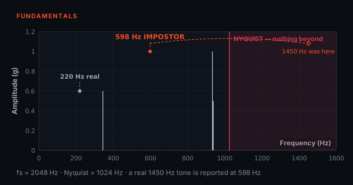
The apparent frequency of an undersampled tone is not random — it is exactly predictable. Take the true frequency f and the sample rate fs: the recorded frequency is |f − fs·round(f/fs)|, always landing somewhere between 0 and Nyquist. Plot that rule and you get a concertina: honest and straight up to fs/2, then folding back down to zero at fs, back up to Nyquist at 1.5·fs, and so on forever.
Two useful landmarks fall straight out of the formula. When the true frequency equals the sample rate exactly, the apparent frequency is zero — every sample lands on the same point of the wave and the record goes flat, which is the wagon wheel appearing to stand still. And just past Nyquist, the apparent frequency comes back down through values that look completely plausible, which is what makes aliases so dangerous in a spectrum.
The playground: slide until it lies
- Watch the white dots, not the red line: they always sit exactly on the grey truth, because an ADC never records a wrong value.
- The thing to stare at is that the red reconstruction passes through every single dot even while it lies. Judged on the stored data — all any analyser ever has — it is a flawless explanation.
- The truth was lost at the instant of sampling, not in processing.
Grey is the true continuous signal. White dots are the samples the ADC stores — notice they always sit exactly on the grey wave, because an ADC never records a wrong value. Red is the sine the analyser reconstructs from those dots alone. While you stay above two samples per cycle, red hugs grey and the reconstruction is honest. Cross the boundary and red detaches into a slower wave that still passes perfectly through every sample.
That last part is the trap worth staring at: even while it lies, the reconstruction never misses a single dot. Judged only by the stored data — which is all any analyser, FFT or algorithm ever has — the red wave is a flawless explanation. The truth was lost at the instant of sampling, not in processing.
Three experiments worth running
First, the slow fall. Set the frequency to 20 Hz and drag the sample rate downward one step at a time. Nothing visible changes for a long while — the dots thin out but the red reconstruction stays glued to the grey truth. The failure is not gradual: at 40 S/s exactly — two samples per cycle — the reconstruction detaches from the grey wave, and every step below that makes it worse. Sampling does not degrade politely; it is honest right up until it isn't.
Second, the standstill. With the rate at 40 S/s, set the frequency to exactly 40 Hz. The apparent frequency reads 0.0 Hz and the red trace goes flat: one sample per cycle, every sample identical. This is the film of a wagon wheel frozen mid-spin — and it is also why a once-per-revolution vibration can vanish entirely from an undersampled record.
Third, the bounce. Hold the rate at 100 S/s (Nyquist 50 Hz) and sweep the frequency up from 40 to 60 Hz. Watch the apparent frequency climb to 50, hit the wall, and walk back down — at a true 60 Hz the analyser reports 40 Hz. Two different inputs, identical files. That symmetry is the folding map from earlier, and you have just traced it by hand.
How this gets caught in the field
- An alias always looks real — a strong, stable line that matches nothing on the machine is exactly what one looks like.
- The diagnostic move costs one re-capture: change only the sample rate. Real components stay put; a real component cannot care what the recorder's clock is doing.
- In the example the shaft line held at 45 Hz while the mystery line jumped from 22 Hz to 150 Hz — both folds of one 490 Hz blade-pass tone above Nyquist.
A representative example, not a specific customer: a maintenance team logs a fan drive with a bare-bones USB logger — no anti-alias filter ahead of the converter — at 512 S/s. The spectrum shows the expected shaft line at 45 Hz, plus a strong, stable line at 22 Hz that matches nothing on the machine: no shaft, no belt, no bearing tone. It looks completely real, because an alias always does.
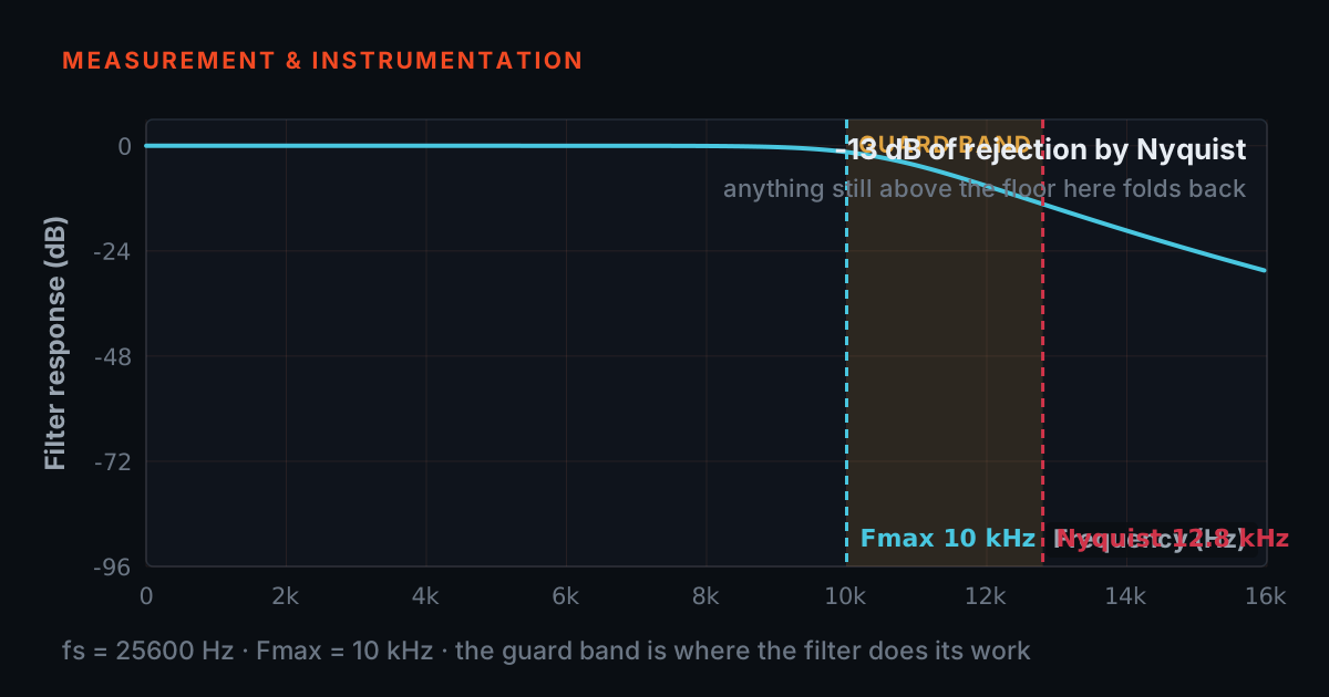
The diagnostic move costs one re-capture: change only the sample rate and see what moves. At 640 S/s the shaft line stays at 45 Hz, but the mystery line jumps to 150 Hz. A real component cannot care what the recorder's clock is doing — so the moving line is an alias. Both positions fold back to the same source, a 490 Hz blade-pass tone sitting above Nyquist in both captures, which a hardware anti-alias filter would have removed before the converter ever saw it. You can replay the whole story in the simulator: it is experiment three, wearing overalls.
Where to go from here
If the playground made the folding rule click, the companion explainer at /blog/sample-rate-fmax-antialias covers the parts a simulator cannot: how Fmax, line count and capture time trade off, and how to read a DAQ datasheet for an honest guard band. The two posts are meant to be read as a pair — one explains, this one lets you break things.
For the underlying theory — sampling, folding, FFT resolution, windowing — TIERA's free primers at 101.tieraonline.in are the place to start: Signal Processing 101 and Accelerometer & DAQ Selection 101. They are free introductory courses, not accredited ISO certifications. When formal, assessed competence matters, the TCAT programme (details at /services) adds structured coursework with proctored examinations at exams.tieraonline.in.
TIERA instruments that do this work.

PhonoVibe Series — Sound & Vibration DAQ
Every model quotes its bandwidth below Nyquist — 20 kHz at 48 kS/s on the D, 60 kHz at 128 kS/s on the Q/O/HD — the honest guard band this playground teaches you to check.
- ADC resolution
- 24-bit, simultaneous sampling on every input
- Sampling
- 48 kHz (D); 128 kHz (Q/O/HD)
- Bandwidth
- 2 Hz – 20 kHz (D); 0.5 Hz – 60 kHz (Q/O/HD)
- Sensor power
- 24 V, 4 mA constant current (IEPE/ICP/CCLD)
- Connectivity
- USB, plug-and-play (Windows 10 / 11)

TVIB — Sound & Vibration Analysis Software
Sample rate, span and lines stay explicitly under your control — so the re-capture-and-see-what-moves test from this post takes a minute, not a support ticket.
- FFT size
- Up to 102,400 points
- Base module
- TSAP201 — free with every PhonoVibe DAQ
- Averaging
- Exponential, linear, peak hold, selectable windowing
- Trial
- 14-day fully-unlocked evaluation licence
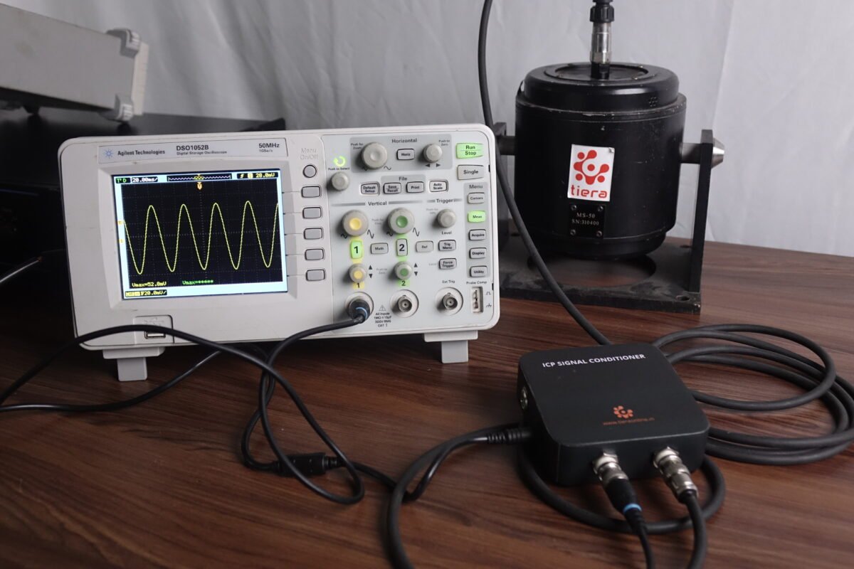
TSP Series IEPE Signal Conditioners
If your recorder is someone else's, TSP 02/04 put the same clean constant-current IEPE excitation ahead of any BNC input — so the front end, at least, is not the weak link.
- Excitation
- 24 VDC, 4 mA constant current
- Frequency response
- 0.5 Hz – 50,000 Hz
- Gain
- 1 (unity)
- Connectors
- BNC in / BNC out
- Channels
- 1 (TSP 02) or 4 (TSP 04)
From the TIERA store
The kit for this job
What we would actually put in front of someone doing the measurement this post describes — not the whole catalogue.
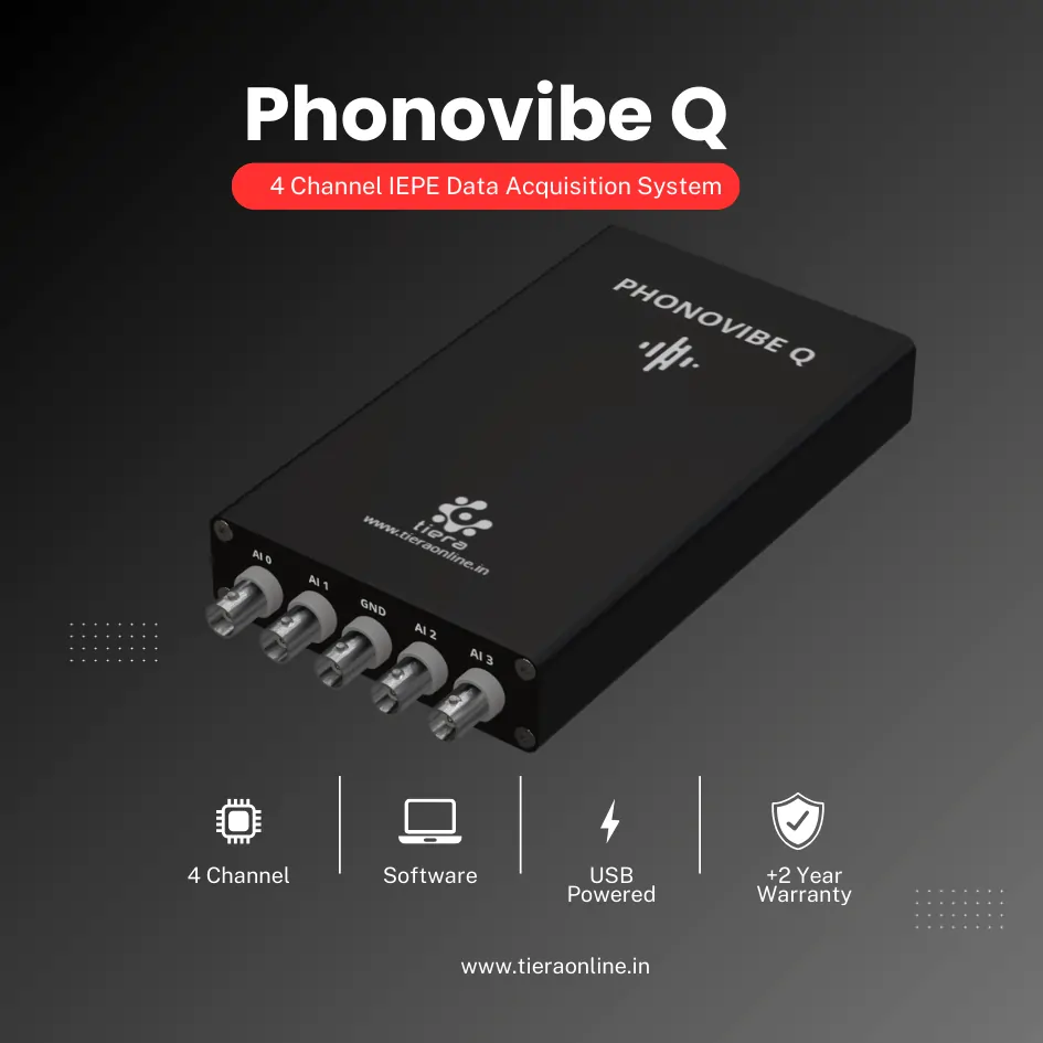 4 Channel IEPE Data Acquisition System – Phonovibe QFour Channels Standard plug & play USB Powered Take data from accelerometers, microphones, hammers, or any other IEPE Sensors T- VIB Software to acquire time waveforms, frequency spectra, overall vibration levels, FRF’s and octave measurements ** Windows 10 or above Operating System ** T-VIB Software base version comes with Time and Spectrum with Post processor TSAP 201. Check out TVIB Software regarding more module options.₹2,88,000View →
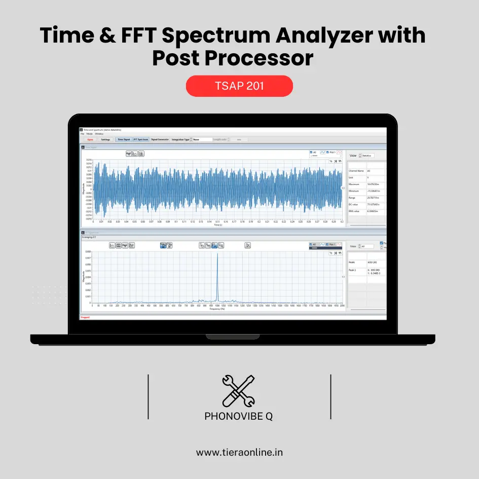 TSAP 201 -Time & FFT Spectrum Analyzer with Post Processor (Phonovibe Q)Use Cases Bump Test Product Development Off route Machine Vibration analysis. Drop Test Product Development & Research₹34,560View →
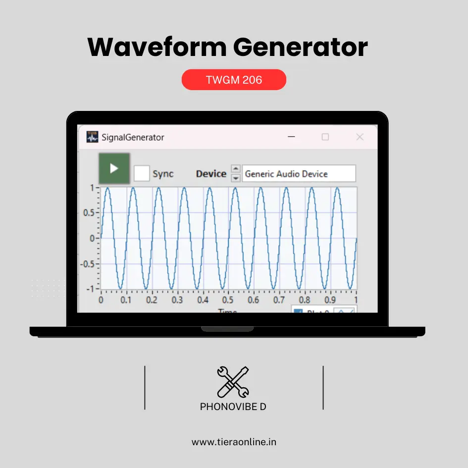 TWGM 206 – Waveform GeneratorUse Cases: Shaker Test for Experimental Modal Analysis₹26,400View →
A front end that keeps the red line on the grey one
The simulator lets you switch aliasing off by moving a slider. On a real machine you cannot — the only protection is hardware: an analogue anti-alias filter ahead of the converter and a sample rate specified with an honest guard band. That is precisely the part of the PhonoVibe series we refuse to compromise: every model quotes its bandwidth below Nyquist (20 kHz at a 48 kHz rate on the 2-channel D; 60 kHz at 128 kHz on the Q, O and 16-channel HD), with 24-bit conversion and simultaneous sampling on every input.
The bundled TVIB TSAP 201 software keeps sample rate, span and lines explicitly under your control — so the re-capture-and-see-what-moves test from this post takes a minute, not a support ticket. And if your recorder is someone else's, the TSP 02 and TSP 04 conditioners provide the same clean 24 V, 4 mA IEPE excitation at unity gain, 0.5 Hz to 50 kHz, ahead of any BNC input.
- PhonoVibe D / Q / O / HD — 2 to 16 channels, 24-bit ADC per channel, simultaneous sampling, IEPE power and TEDS on every model
- Bandwidth specified below Nyquist on every datasheet — the guard band you can check yourself
- TVIB TSAP 201 bundled: sample rate, Fmax, lines and averaging under explicit control
- TSP 02 / TSP 04 IEPE signal conditioners for third-party DAQs and recorders
Where this sits on the TIERA learning ladder.
The theory behind this article is covered free, in full, by the TIERA 101 primers: Signal Processing 101, Accelerometer & DAQ Selection 101. They are self-paced, interactive, and end in an exam and a certificate.
The free 101 primers cover the sampling and folding theory behind this playground; the formal TCAT programme (see /services) adds structured coursework and proctored examinations at exams.tieraonline.in for teams that need assessed, certificated competence.
TIERA 101 is a free introductory primer, not an accredited ISO certification, and its hours do not count towards the formal training ISO 18436 requires.