How an AI Condition-Monitoring System Is Actually Built
The end-to-end engineering of an AI condition-monitoring system, honestly: instrumentation that sets the ceiling, a baseline wide enough to trust, features you can audit, why real deployments are anomaly detection rather than fault classification, thresholds and persistence rules, and the drift and re-baselining that fill the years afterwards.
The pipeline at a glance — and where the ceiling is set
- The ceiling is set at the front of the chain, before any model exists: capture at a rate sized for shaft speed alone and the earliest bearing evidence is simply not in the data.
- The model is the fourth link, not the first, and rarely the one that decides whether the system works.
- Same point, same mounting, same acquisition settings, a tacho reference, and the operating state logged beside every capture — that is what makes a month-one capture comparable with a month-eighteen one.
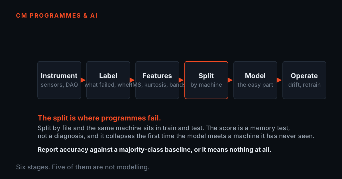
Strip the marketing away and an AI condition-monitoring system is a chain of seven decisions: what to sense, how to capture it, what numbers to compute from it, what 'normal' means, how to score departures from normal, when a score becomes an alarm, and who does what when it does. The model — the part every brochure leads with — is one link, and rarely the one that decides whether the system works.
The ceiling is set at the front of the chain, before any model exists. A rolling-element bearing announces itself as short impacts that excite resonances in the kilohertz range, so the sample rate and anti-alias filtering must keep that band — capture at a rate sized for shaft speed alone and the earliest fault evidence is simply not in the data, and no model can recover it. Mounting works the same way: a stud-mounted accelerometer holds its bandwidth; a loosely placed magnet or a hand-held probe rolls off exactly where the interesting energy lives, and moving the sensor a few centimetres between visits changes the signal more than most early faults do.
Consistency is the least glamorous requirement and the most binding one. Same measurement point, same mounting, same acquisition settings, a tachometer reference for speed, and the operating state (speed, load, temperature) recorded alongside every capture. A 24-bit, simultaneously-sampled chain with sensor identification (the routine PhonoVibe-class setup, with TEDS so the sensor's own sensitivity travels with it) is not a luxury here — it is what makes a capture in month one comparable with a capture in month eighteen, which is the entire premise of the exercise.
The baseline: 'normal' is whatever you showed the model
- Every operating state the baseline missed will later score as an anomaly while the machine is perfectly healthy.
- One week at one load is not wrong, it is narrow — and narrowness converts directly into false alarms.
- Without speed and load logged next to every capture, nobody can later separate machine changed from operation changed, and that question is the whole game.
An anomaly model has no concept of a healthy machine. 'Normal' is defined operationally: it is the span of the data used to fit the baseline, nothing more. So the real engineering question is coverage — which speeds, which loads, which valve line-ups, which ambient temperatures did the baseline actually see? A machine on a VFD runs a range of speeds; a pump sees seasonal water temperatures; a compressor loads and unloads. Every one of those is a different 'normal', and every one the baseline missed will later score as an anomaly while the machine is perfectly healthy.
This is why a baseline recorded over one week at one load is a trap. It is not wrong — it is narrow, and narrowness converts directly into false alarms. A defensible baseline is usually weeks to a few months of captures, deliberately spanning the duty cycle: multiple speeds, low and high load, cold start and hot running, and ideally a note of anything unusual that happened while it was recorded. If an operating state cannot be covered yet (the winter condition, in summer), the honest options are to wait, or to deploy knowing that state will alarm falsely once and extend the baseline when it does.
There is a design choice hiding here too: either the baseline is wide enough to absorb all duty points into one model, or captures are segmented by operating state — a per-speed-band baseline, selected using the recorded tacho and load metadata. Segmentation is more work and much easier to defend, because it stops the model blaming the machine for what the process did. Either way, the metadata is not optional: without speed and load logged next to every capture, no one can later separate 'machine changed' from 'operation changed', and that question is the whole game.
Features versus raw waveform: buying auditability
Each capture has to become numbers the model can watch. One school hands the model raw waveform windows and lets a deep network learn its own representation. The other computes engineered features first — overall RMS, crest factor, energy in defined frequency bands (1x and harmonics, a bearing-tone region, gear-mesh sidebands), envelope-spectrum band power at the bearing defect frequencies, sideband ratios around mesh — and lets a much simpler detector watch that short vector. These are the same quantities a vibration analyst reads off a spectrum, which is precisely the point.
The trade is real and worth stating plainly. Raw-waveform deep models are more flexible and can, with enough data, find patterns nobody thought to encode — but they need far more data than one machine's healthy history usually provides, and when the score rises, nobody can say why. The feature path may flag a little later, but every alarm decomposes into physics: the envelope band moved, or crest factor jumped, or 2x grew against 1x. In a plant, where an alarm's first audience is a sceptical engineer deciding whether to strip a machine, that auditability is usually worth more than the last fraction of sensitivity. This trade-off is examined at more length in the companion piece on what anomaly detection can and cannot claim.
In practice the features come from the same analysis toolchain the humans use — in a TVIB-class workflow, the narrowband FFT with band and sideband cursors and crest factor are computed and exported per capture — so the model and the analyst are looking at the same quantities. When they disagree, that shared vocabulary is what makes the disagreement resolvable.
Choosing the method: the data you have decides, not the ambition
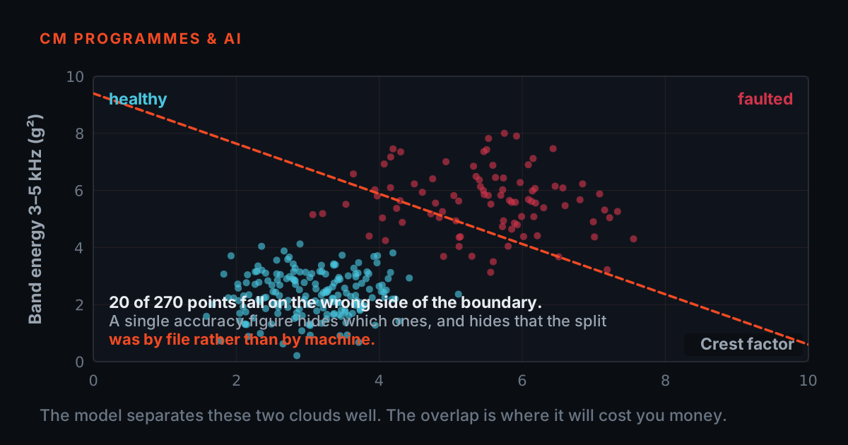
There are two families of model, and the choice between them is not really a modelling decision — it is a statement about what data exists. Supervised classification learns to name faults: it needs many labelled examples of each fault type, on relevantly similar machines, across severities. One-class anomaly detection learns only the shape of healthy data — a statistical envelope around the baseline feature vectors — and scores how far each new capture sits from it. It never names anything; its entire vocabulary is 'not normal, this much'.
Almost nobody operating real machines has the labelled fault library that classification requires. Plants run machines to avoid faults; the failures that do occur are rare, often mixed-mode, and get labelled weeks later from a work order, if at all. Fault data borrowed from other machines or public datasets transfers poorly, because a bearing signature is entangled with the specific machine, mounting, and speed it was recorded on. So the honest default — and what most credible deployments actually run — is one-class anomaly detection trained on the plant's own healthy history. The model family itself matters less than the inputs: on a well-built feature set, simple distance-based or density-based one-class methods are hard to beat and easy to interrogate.
Classification is not a myth; it is a second stage with a real entry price: labelled fault recordings. Where those come from — and what they buy — is the last section of this post.
Thresholds, persistence, and validating without a labelled test set
- The threshold comes from the baseline's own score distribution, paired with a persistence rule — M of the last N captures above the line, not one excursion.
- That single rule removes most false alarms at the cost of reacting a few captures later, which for faults developing over weeks is overwhelmingly the right trade.
- You cannot measure a detection rate without faults. You can measure a false-alarm rate on held-out healthy data, and that is the number to ask for.
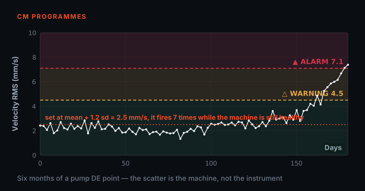
A score stream is not a monitoring system until something turns it into an alarm, and this is where good builds get deliberately boring. The threshold is set from the baseline itself — from the distribution of scores the healthy data produces, placed high enough that ordinary variation stays under it — and it is paired with a persistence rule: the alarm fires only when some number of consecutive captures (or M of the last N) stay above the line. A single excursion is noise, a sensor knock, or a process transient; a sustained excursion is information. That one rule removes most false alarms at the cost of reacting a few captures later, and for faults that develop over weeks the trade is overwhelmingly right. The economics of exactly where to put the lines — and what each false alarm costs in team trust — are explored interactively in the alarm-threshold simulator.
Then comes the question every buyer should ask and few do: how was this validated, given that there is no labelled test set? You cannot measure a detection rate without faults to detect. What you can measure honestly is the false-alarm rate: hold out a slice of healthy data the model never saw — ideally later in time, and including duty points at the edge of coverage — and count how often the alarm logic fires on it. You can also rehearse the system against events with known causes: a deliberate speed change, a sensor remount, a maintenance intervention, and confirm the score and the operating-state metadata tell a consistent story. What no one can honestly tell you, before real faults occur, is the probability the system catches the next one. Treat any vendor quoting that number without a labelled test set with suspicion.
Deployment reality: drift, re-baselining, and who acts on the alert
- Drift makes the score climb because normal moved away from the baseline, not because the machine moved away from normal.
- Re-baseline only after a known event — overhaul, sensor change, verified duty change — and only after a human has looked at a spectrum and pronounced the machine healthy.
- An automatic re-baseline can quietly learn a developing fault as the new normal, which defeats the entire purpose. Archive the old baseline rather than deleting it.
The model that goes live is a snapshot of a machine that will not stay still. Seasons change intake temperatures; production changes loads; wear changes the machine slowly in ways that are real but not urgent; a bearing replacement or realignment changes it overnight in ways that are healthy. All of this is concept drift: the score creeps upward not because a fault is developing but because 'normal' has moved away from the baseline. Left alone, drift manufactures alarms until the team stops believing them — the alarm-fatigue failure mode, where the one alert that matters dies in a full inbox.
The countermeasure is re-baselining, and it needs discipline in both directions. Re-baseline too rarely and false alarms grow; re-baseline too eagerly — worst of all, automatically — and the system can quietly learn a developing fault as the new normal, which defeats the entire purpose. The workable rule: re-baseline only after a known event (overhaul, sensor change, verified duty change), and only after a human has checked the current condition — a spectrum and envelope look, not a glance at the score — and pronounced it healthy. The old baseline is archived, not deleted; the divergence between old and new is itself a record of how the machine has moved.
Which surfaces the part no architecture diagram shows: an alert is only worth what the response to it costs and catches. Someone specific — named, trained, with time allocated — has to receive the flag, check operating state before touching the machine, take a proper measurement, and decide what the score means. The model says 'look here'; the meaning is assigned by a person who can read a spectrum. What the model can and cannot claim at that moment is the subject of the companion post on the limits of anomaly detection — the short version is that an anomaly score is a prompt to investigate, never a diagnosis, and a deployment staffed as if it were a diagnosis machine will fail on its first ambiguous alarm.
A representative build, end to end
A representative deployment, not a specific customer: a plant picks six cooling-water pumps — enough to matter, few enough to do properly. Accelerometers go on drive-end and non-drive-end bearing housings, stud-mounted after a bandwidth check; a tacho reference is wired in; capture settings are fixed once and written down. Eight weeks of baseline follow, deliberately spanning the VFD speed range and both summer duty points, with speed and load logged against every capture. Features are band energies, crest factor, and envelope band power at the fitted bearings' defect frequencies. A one-class model is fitted per speed band; the threshold comes from the held-out tail of the healthy scores; the alarm rule is three consecutive captures above the line.
The first month produces exactly the failures this post predicts: a duty change that was never baselined trips the alarm, the operating-state check catches it in minutes, and the baseline is extended rather than the threshold raised. Months later a score climbs and stays climbed across two weeks with no matching process change. The technician connects a portable analyser, and the envelope spectrum shows non-synchronous lines at a bearing defect frequency. The model never said 'bearing' — it said 'not normal, persistently, at this measurement point', and a person with a spectrum said the rest. The repair is scheduled instead of suffered. No accuracy percentage, uptime figure, or cost saving is attached to this story, because inventing one is exactly the habit this post is arguing against.
Where labelled fault data actually comes from — and what it buys
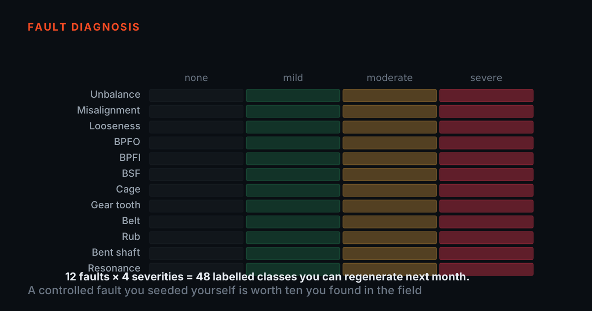
If the system should ever do more than say 'not normal' — rank candidate faults, estimate severity, pre-sort alarms for the analyst — it needs training data where the fault is genuinely known. The field will not provide it: real failures are rare, labels get reconstructed weeks later from work orders, and teardowns routinely find several damage mechanisms at once with no way to say which one the recording captured. The place labels actually come from is a fault simulator, where the order of events is reversed: the fault is installed and documented before the signal exists. On a rig like the TMFSS, the same seeded defect — unbalance, misalignment, an outer-race bearing fault, looseness, gear damage — is run across speeds and loads on demand, and an accelerated-bearing-wear kit turns a single good-or-bad pair into a staged degradation sequence, which is what severity estimation needs.
What that buys is precise but bounded. Simulator data trains and validates the fault-recognition layer — the classifier that turns 'anomalous' into 'consistent with a bearing fault' — and it hardens the feature set, by showing which features actually move for which faults on a machine where the truth is known. What it does not do is replace the plant's own baseline: a simulator tells you what a fault looks like, not what your pump in your plant looks like on a healthy Tuesday. The two datasets answer different questions, and a serious build uses both. The full lab workflow for generating that labelled data — the rig, the capture chain, the metadata — is covered in the companion note on ML/AI algorithm development for predictive maintenance.
There is one discipline that decides whether the number that comes out of that classifier means anything, and it is not a modelling choice. Split the data by physical asset, never by run, file or segment. Cut one ten-minute recording into segments and shuffle them across train and test and the model memorises that machine's mounting, resonances and background — and reports an accuracy that measures your split, not your algorithm. Splitting by run is not enough either: two runs on the same rig share all of it. And report the majority-class baseline next to every score, because on data that is mostly healthy, a model that always answers 'healthy' scores whatever the healthy fraction is. The full lab workflow — capture, metadata, group-aware hold-out design, and what to report — is covered in the companion note on building a CM dataset that does not lie to your model.
The theory under all of this is learnable for free: the TIERA 101 primers at 101.tieraonline.in — including AI Condition Monitoring 101 and Measurement Setup 101 — cover it without hype; they are free primers, not accredited ISO certification. For teams that need assessed, certification-grade analyst skills behind the human-in-the-loop, the TCAT programme described at /services adds structured coursework with proctored exams at exams.tieraonline.in.
TIERA instruments that do this work.

TMFSS — Machinery Fault Signature Simulator
The labelled ground truth of section eight: seeded faults installed and documented before the signal is captured, repeatable across speeds and loads — including staged bearing-wear sequences via add-on kits.
- Faults (Macro)
- 30+ base kit, extensible with add-on kits
- Speed control
- VFD with WiFi software
- Tachometer
- Built-in, analog output
- Foundation
- Solid rigid base — repeatable signatures
- Warranty
- 1 year; AMC available

PhonoVibe Series — Sound & Vibration DAQ
The capture consistency the baseline depends on — the same 24-bit, simultaneously-sampled, calibrated chain making month one comparable with month eighteen.
- ADC resolution
- 24-bit, simultaneous sampling
- Sensor power
- IEPE / ICP / CCLD — 24 V, 4 mA
- Sampling
- 48 kHz (D) · 128 kHz (Q / O / HD)
- TEDS
- Supported
- Calibration
- Factory certificate, 1-year validity

TVIB — Sound & Vibration Analysis Software
Computes the auditable features of section three — narrowband FFT with band and sideband cursors, crest factor — so the model and the analyst watch the same quantities.
- FFT size
- Up to 102,400 points
- Cursors
- Harmonic, band and sideband — time & frequency
- Base module
- TSAP201 — free with every PhonoVibe
- Trial
- 14-day fully-unlocked evaluation licence
From the TIERA store
The kit for this job
What we would actually put in front of someone doing the measurement this post describes — not the whole catalogue.
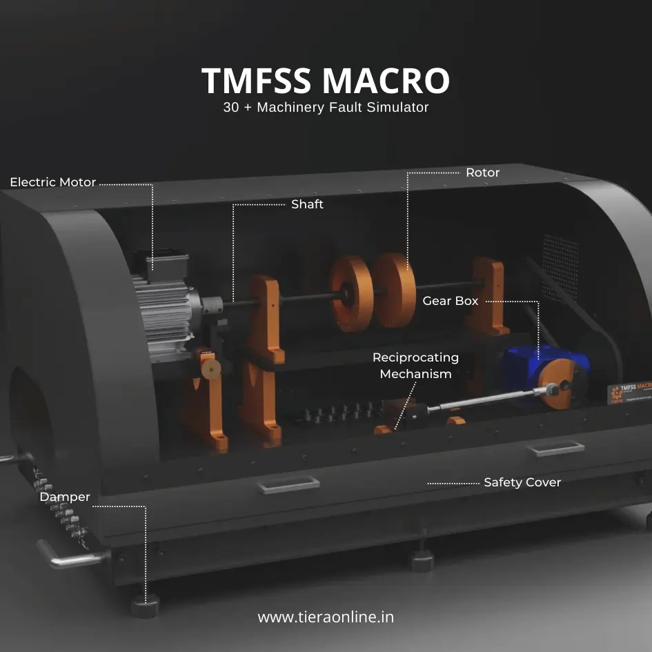 Machinery Fault Signature SimulatorTiera’s Machine Fault Simulator (TMFSS) is a valuable tool for industries and researchers, simulating over 30 real-world faults such as: Bearing faults: outer race defects, inner race defects, cage defects. Motor faults: stator faults, rotor faults, electrical unbalance. Gearbox faults: gear wear, misalignment, gear tooth damage. And more.₹13,53,600View →
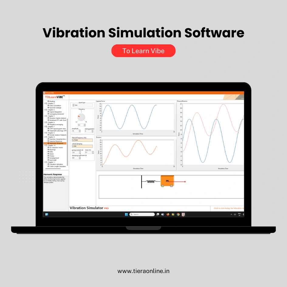 To Learn Vibe -Vibration Simulation Software Basic (Yearly Subscription)For comprehensive vibration analysis training, start with our To Learn Vibe software. Covering everything from basic to advanced vibration concepts, this software is designed to kickstart your career and enhance your expertise. Perfect for mastering fundamental and advanced vibration analysis, To Learn Vibe equips you with the knowledge and skills needed to excel in the field of vibration engineering.₹34,560View →
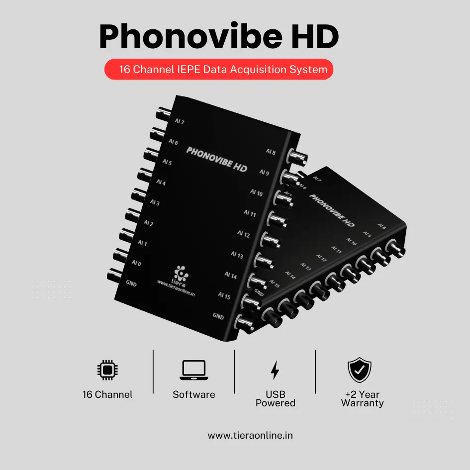 16 Channel IEPE Data Acquisition System-Phonovibe HDSixteen-Channel Data Acquisition System Plug & Play USB Powered Compatible with accelerometers, microphones, hammers, and other IEPE sensors T-VIB Software for time waveforms, frequency spectra, vibration levels, FRFs, and octave measurements Base version includes Time and Spectrum with TSAP 201 post-processor Explore additional modules with T-VIB Software₹7,20,000View →
Use cases
Where this shows up in the field
TIERA sells the parts of this pipeline you cannot download — not a fault-naming oracle.
After eight sections of 'the model is the easy part', it would be strange to end by selling you a model. TIERA builds the layers underneath: capture hardware consistent enough that month one and month eighteen are comparable, analysis software that computes the auditable features this post is built on, a fault simulator that manufactures the labelled ground truth the field will never give you, and training tools for the analyst who turns a score into a decision.
If you are building this pipeline — or evaluating someone who claims to have — these are the pieces worth putting money into first.
- TMFSS fault signature simulator — 30+ fault types in the Macro base kit, installed and documented before capture, repeatable across speeds and loads; add-on kits include accelerated bearing wear for staged severity sequences. This is where labelled fault data comes from.
- PhonoVibe DAQ series — 24-bit, simultaneous sampling on every channel, IEPE sensor power with TEDS recognition and a factory calibration certificate: the capture consistency the baseline depends on.
- TVIB analysis software — narrowband FFT with band and sideband cursors, crest factor, filtering and averaging: the engineered features of section three, computed and exportable per capture.
- To-Learn Vibe — 100+ simulated fault scenarios to train the human-in-the-loop, so the person answering the alarm has practised naming faults before a model starts raising them.
Where this sits on the TIERA learning ladder.
The theory behind this article is covered free, in full, by the TIERA 101 primers: AI Condition Monitoring 101, Measurement Setup 101. They are self-paced, interactive, and end in an exam and a certificate.
TCAT adds structured, instructor-led coursework and proctored certification exams at exams.tieraonline.in — turning primer-level understanding of this pipeline into an assessed, industry-recognised analyst skillset.
TIERA 101 is a free introductory primer, not an accredited ISO certification, and its hours do not count towards the formal training ISO 18436 requires.