What AI Can and Cannot Tell You About a Machine
Anomaly detection is genuinely useful: it says 'this is not normal' earlier than a human round can. But it does not name the fault, and it inherits every bias in the baseline it learned. An honest look at scores, thresholds, false alarms, and why labelled data matters.
'Not normal' is useful — and it is all the model says
- A score of 0.91 means look here. It does not mean bearing, misalignment or a loose cable — naming the fault still takes defect frequencies and someone who can read a spectrum.
- What the model actually buys you is timing: it watches every hour, so it can notice a drift long before the next manual route comes round.
An anomaly detector does one thing: it learns what a machine's signals look like during normal running, and it raises a score when new data stops looking like that. This is genuinely valuable. Machines drift into failure over days and weeks, and a model that watches every hour can notice a change long before the next manual measurement route comes around.
But be clear about what the score contains. A reading of 0.91 does not say bearing, does not say misalignment, does not say loose sensor cable. It says: look here. Naming the fault still takes physics — defect frequencies, envelope analysis, an analyst who knows what a 1x-spaced sideband means. An anomaly score is a prompt to look, not a diagnosis, and every deployment that treats it as more than that eventually gets burned.
The baseline is the model — and it inherits every bias
- 'Normal' is only the speeds, loads, season and mounting position the model happened to see. An unfamiliar duty point and a genuine fault are mathematically the same thing to it: far from what it learned.
- Log speed, load and measurement setup with every capture. That metadata is what later answers the only question that separates a false alarm from a find — did the machine change, or did the operating condition?
Anomaly detection has no idea what a bearing is. 'Normal' is defined entirely by the data the model saw during training: those speeds, those loads, that season, that sensor in that mounting position. If the baseline was recorded in winter at one duty point, then a hot afternoon at a higher pump speed is, mathematically, an anomaly — the model cannot tell an unfamiliar operating condition from a fault, because both are simply 'far from what I learned'.
This is why the boring metadata matters as much as the waveform. Recording speed, load, and measurement setup alongside every capture — a tachometer or speed reference logged alongside simultaneous multi-channel sampling, the kind PhonoVibe's parallel-sampled inputs make straightforward — is what later lets you ask the only question that separates a false alarm from a find: did the machine change, or did the operating condition change?
Thresholds, false alarms, and alarm fatigue
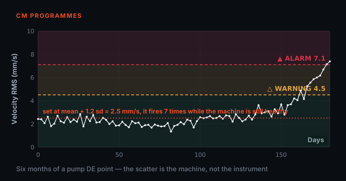
- The shape of an excursion tells you more than the crossing does: a spike that is back at baseline within hours is an operating change, a climb that persists week after week is a machine.
- Check every alarm against the operating state before you check it against the machine — it is the cheaper of the two checks and it settles most of them.
Every anomaly system needs a threshold, and every threshold is a trade. Set it low and you catch faults early but flag every speed step and process change; set it high and the panel stays quiet until the fault is loud. The trend below shows the two events that matter: a sharp spike when the operating condition changed — over in hours, back to baseline, no fault — and a slow, sustained rise that keeps climbing week after week. The shape of the excursion carries more information than the fact of crossing the line.
False alarms are not free. Each one sends someone to a healthy machine, and each wasted trip spends a little of the team's trust. After enough of them, flags get acknowledged without being investigated — alarm fatigue — and the one alert that mattered dies in a full inbox. A practical rule: act on sustained trends, and check every alarm against the operating state before checking it against the machine.
Features vs raw waveform: pay for accuracy with auditability
There are two ways to feed a machine signal to a model. Hand it raw waveform windows and let a deep network find its own patterns — flexible, but data-hungry, and when the score rises nobody can say why. Or compute engineered features first — band energy, envelope-spectrum lines at bearing defect frequencies, crest factor, sideband ratios — and let a simpler detector watch those. The feature path usually detects a little later, but it fails in ways an engineer can inspect.
That auditability is worth a lot in practice. TVIB computes and exports exactly these quantities — narrowband FFT, crest factor, band and sideband cursors — so when an alarm fires you can open the feature that moved and see, for instance, that energy rose in the bearing band. The alarm stops being a mystery score and becomes the first line of the diagnosis.
A representative deployment, not a specific customer
A plant puts an anomaly model on a cooling-water pump, trained on three months of normal running. In summer, operations raises the VFD speed to meet load — and the score spikes. The baseline never contained that speed, so to the model the healthy pump at the new duty point is an anomaly. A technician walks out, finds nothing wrong, and the team retrains the baseline to include the new condition. That trip was the cost of a biased baseline, not a model bug.
Weeks later the score begins a slow, sustained climb with no matching change in operating state. This time the flag earns its keep: a technician connects a two-channel PhonoVibe D, and the narrowband spectrum in TVIB, read against the band and sideband cursors, shows non-synchronous lines at a bearing defect frequency. The fault now has a name, the repair gets scheduled instead of forced, and the division of labour is exactly right — the model prompted the look, the measurement and the analyst named the fault.
Why a labelled fault library beats scraped field data
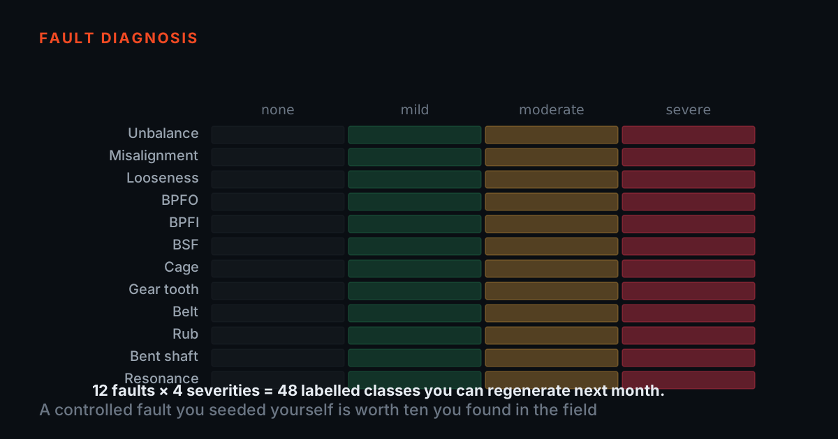
If you want the model to do more than say 'not normal' — to rank likely fault types, or estimate severity — you need training data where the fault is actually known, and in a working fleet that is the scarce resource: failures are rare by design (that is the whole point of maintenance), so collecting enough labelled examples of any one fault to train a classifier means living through a lot of unplanned downtime first. Scraped field data makes the shortage worse, not better: labels get assigned weeks after capture from work orders and teardowns, real failures mix several mechanisms at once, and speed and load drift between recording and inspection. A simulator reverses the order: on a TMFSS the fault is installed and documented before the signal is captured, the same defect can be repeated across speeds and loads, and the accelerated-bearing-wear kit lets you record a staged degradation sequence rather than a single good-or-bad pair. To-Learn Vibe trains the analyst side of that same problem: the trainee diagnoses a simulated fault against a known answer, building exactly the pattern-recognition skill an anomaly flag still needs once it reaches a human.
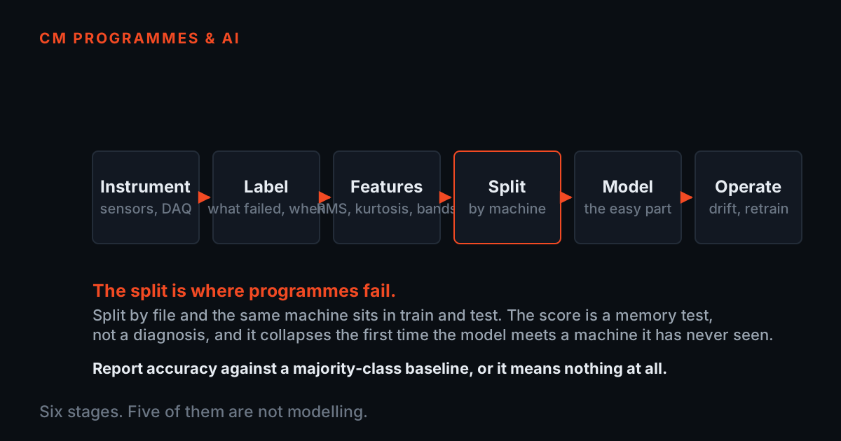
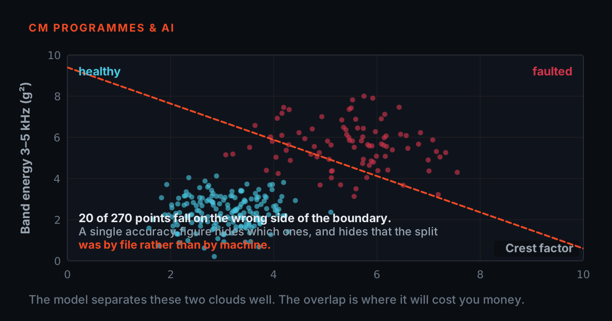
There is a trap on the other side of a good dataset, and it is the reason published accuracy figures on machine-fault data are usually too good to be true. Once you have many recordings of the same fault you have to split them into training and test sets — and if you split by file, or by run, then segments of one recording of one bearing land on both sides of the split. The model scores ninety-nine per cent because it has learned to recognise that particular bearing on that particular afternoon, not the fault. Split by physical asset instead: every recording of a given bearing, shaft or gearbox goes wholly into training or wholly into test, and the number you get is the number you will see on the next machine.
Then insist the score is quoted against the majority-class baseline. On a fleet where ninety-five per cent of readings are healthy, a model that answers 'healthy' every single time is ninety-five per cent accurate and worth precisely nothing — so a bare accuracy figure carries no information until you know what guessing would have scored. If a vendor shows you an accuracy number without saying how the split was made and what the baseline was, the number is not evidence, and asking those two questions is the fastest way to find out whether anyone on the other side has done this before.
This post is the second half of a pair: the earlier note on building predictive-maintenance datasets, at /blog/ml-ai-predictive-maintenance, covers how that labelled data gets generated and captured; this one covers what the trained model can honestly tell you afterwards. For the theory underneath both, the free primers at 101.tieraonline.in include AI Condition Monitoring 101 — a free primer, not an accredited certification — and TIERA's formal TCAT programme, detailed at /services, adds structured coursework with proctored exams at exams.tieraonline.in.
TIERA instruments that do this work.

TMFSS — Machinery Fault Signature Simulator
Generates fault data where the label is set before the signal exists — the ground truth an anomaly detector has to be trained and tested against.
- Faults (Macro)
- 30+ base kit, extensible with add-on kits
- Speed control
- VFD with WiFi software
- Tachometer
- Built-in, analog output
- Foundation
- Solid rigid base — repeatable signatures across sessions
- Warranty
- 1 year; AMC available

PhonoVibe Series — Sound & Vibration DAQ
Consistent, calibrated capture — so the baseline the model learns and the follow-up it scores are actually comparable recordings.
- Resolution
- 24-bit ADC, simultaneous sampling on every input
- Channels
- 2 / 4 / 8 / 16 (D / Q / O / HD)
- Sensor power
- IEPE / ICP / CCLD — 24 V, 4 mA; TEDS recognition
- Calibration
- Factory certificate, 1-year validity

TVIB — Sound & Vibration Analysis Software
The engineered features and cursors that keep an analyst in the loop — turning 'this is not normal' into 'energy rose in the bearing band'.
- FFT size
- Up to 102,400 points
- Cursors
- Harmonic / band / sideband
- Base module
- TSAP201 — free with PhonoVibe
- Trial
- 14-day fully-unlocked evaluation licence
From the TIERA store
The kit for this job
What we would actually put in front of someone doing the measurement this post describes — not the whole catalogue.
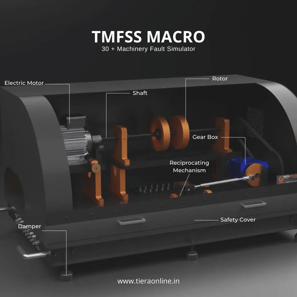 Machinery Fault Signature SimulatorTiera’s Machine Fault Simulator (TMFSS) is a valuable tool for industries and researchers, simulating over 30 real-world faults such as: Bearing faults: outer race defects, inner race defects, cage defects. Motor faults: stator faults, rotor faults, electrical unbalance. Gearbox faults: gear wear, misalignment, gear tooth damage. And more.₹13,53,600View →
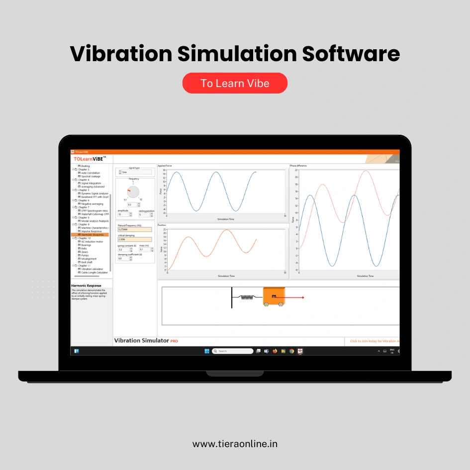 To Learn Vibe -Vibration Simulation Software Basic (Yearly Subscription)For comprehensive vibration analysis training, start with our To Learn Vibe software. Covering everything from basic to advanced vibration concepts, this software is designed to kickstart your career and enhance your expertise. Perfect for mastering fundamental and advanced vibration analysis, To Learn Vibe equips you with the knowledge and skills needed to excel in the field of vibration engineering.₹34,560View →
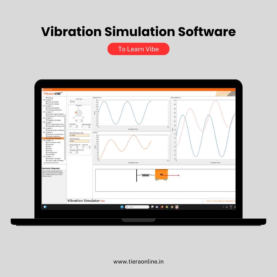 To Learn Vibe -Vibration Simulation Software PRO (Yearly Subscription)For comprehensive vibration analysis training, start with our To Learn Vibe software. Covering everything from basic to advanced vibration concepts, this software is designed to kickstart your career and enhance your expertise. Perfect for mastering fundamental and advanced vibration analysis, To Learn Vibe equips you with the knowledge and skills needed to excel in the field of vibration engineering.₹86,400View →
Use cases
Where this shows up in the field
The model says 'look here'. TIERA supplies everything that happens next.
TIERA does not sell a model that names your faults — after this post, you would not trust one that claimed to. What we build is the rest of the loop: a simulator that generates fault data where the label is set before the signal exists, a measurement chain that captures it (and your field data) consistently enough to compare, and the analysis and training tools that keep a human who can read a spectrum in the loop.
If you are building or buying anomaly detection, that is the part worth spending on first: ground truth to train and test against, capture you can audit, and an analyst who can turn a score into a diagnosis.
- TMFSS fault signature simulator — 30+ fault types in the Macro base kit, installed and documented before capture, repeatable across speeds and loads; add-on kits include accelerated bearing wear for staged degradation sequences.
- PhonoVibe DAQ series — 24-bit, simultaneous sampling on every input, IEPE sensor power with TEDS recognition, and a factory calibration certificate (1-year validity), so baseline and follow-up captures are actually comparable.
- TVIB analysis software — narrowband FFT with harmonic, band, and sideband cursors, filtering and averaging: the engineered features that turn 'score: 0.91' into 'energy rose in the bearing band'.
- To-Learn Vibe — 100+ simulated fault scenarios for the analyst side of the loop, so the person answering the flag has practised naming faults before a model starts raising them.
Where this sits on the TIERA learning ladder.
The theory behind this article is covered free, in full, by the TIERA 101 primers: AI Condition Monitoring 101. They are self-paced, interactive, and end in an exam and a certificate.
TCAT adds structured, instructor-led coursework and proctored certification exams at exams.tieraonline.in — turning primer-level intuition into an assessed, industry-recognised analyst skillset.
TIERA 101 is a free introductory primer, not an accredited ISO certification, and its hours do not count towards the formal training ISO 18436 requires.