


Building a Condition-Monitoring Dataset That Does Not Lie to Your Model
Most published 99% accuracies in machinery diagnostics are leakage. Split segments from the same recording across train and test and the model memorises the machine, not the fault — and the number it reports is a measurement of your split, not of your algorithm.
Why real fault data is scarce, and what people do about it
Machines that matter are maintained. They are supposed not to fail, and when they do, the priority is getting them running again — not instrumenting the failure for a dataset. So the data that exists is overwhelmingly healthy, the faults that do occur are unlabelled or labelled after the fact from a work order, and the severe cases you most want are the rarest of all.
Three routes out, each with an honest cost. Public datasets are convenient and small, and everyone has already fitted them — a result on one is a sanity check, not evidence. Field data is the real distribution but arrives unlabelled, imbalanced and slowly. Seeded-fault rigs give you labelled, balanced, severity-graded data quickly, at the cost of being a rig rather than a plant.
In practice serious work uses all three: a rig to develop and stress the method, public data to compare against others, and field data to find out what actually transfers. The mistake is stopping at the first and reporting its numbers as if they were the third.
The leakage that produces 99% accuracy
Here is the failure, and it is close to universal in published machinery-diagnostics results.
You record ten minutes from a machine with a bearing fault. You cut it into 1-second segments and get 600 samples. You shuffle them and split 80/20 into train and test. You train a classifier and it scores 99%.
That number is meaningless. Segments 341 and 342 came from the same recording, seconds apart, on the same machine, with the same mounting, the same background noise, the same speed and the same sensor. The model did not learn what a bearing fault sounds like. It learned what that recording sounds like — and then you tested it on more of the same recording.
Show it a different machine and it collapses, which is exactly the moment your project is discovered to be worthless — usually in front of a customer.
The fix is to split by physical asset. Every segment from a given machine goes entirely into train, or entirely into test, never both. Splitting by run or by file is not enough on its own either: two runs on the same machine share the mounting, the resonances and the background, so the same memorisation is available. The unit of independence is the asset.
Where you genuinely have only one machine, say so and report the result as what it is — a within-machine result that demonstrates the method can separate the classes, with no claim about generalisation. That is a defensible thing to publish. A shuffled 99% is not.
Vary what the field varies
A dataset recorded at one speed, one load, one temperature and one mounting produces a model that works at one speed, one load, one temperature and one mounting. Plants do not oblige.
Vary speed deliberately, including the fixed-speed case, because most industrial machines are direct-on-line and never change speed at all — a method that needs a run-up is unusable on them. Vary load, because load changes both the fault's excitation and the structure's response. Vary mounting, because the mount sets the usable bandwidth and a model trained only on stud-mounted data will fail on magnet-mounted field records. Vary severity, because a classifier trained only on severe faults detects nothing early, which is the entire point of condition monitoring.
And include the awkward classes: multiple simultaneous faults, and — most neglected of all — bad records. Clipping, dropouts, a dead channel, line-frequency pickup, aliasing. A model that has never seen a corrupted record will confidently classify one, and in production corrupted records are far more common than rare faults.
Features, and the baseline that keeps you honest
Standard condition-monitoring features are a strong starting point and remain competitive against learned representations on small datasets: RMS, peak, crest factor, kurtosis, spectral band energies keyed to the actual fault frequencies (BPFO, BPFI, BSF, FTF, gear mesh, shaft orders), and envelope-spectrum band energy. They have the large advantage of being interpretable, so when the model fires you can say what fired it.
Two disciplines matter more than the feature choice. Fit every transform on training data only. Standardisation, PCA, feature selection — compute the parameters on train and apply them to test. Fitting a scaler on the whole dataset before splitting leaks test statistics into training, and it is the second most common way a result gets inflated.
Always report a baseline. If 70% of your samples are healthy, a model that predicts 'healthy' every time scores 70%. Any accuracy figure without the majority-class baseline beside it is uninterpretable. In fact, prefer not to headline bare accuracy at all: on imbalanced condition-monitoring data it is the metric that most flatters a useless model. Per-class precision and recall, a confusion matrix, and PR-curve average precision say what is actually happening — particularly for the rare severe class you care most about.
If you are doing prognostics, the bar is higher again
Remaining-useful-life work needs run-to-failure trajectories, which are far more expensive to obtain than fault classification data — you need the whole degradation, not a snapshot.
Two properties make a health index worth trending: monotonicity (it should mostly move one way as damage accumulates) and trendability (it should correlate with time to failure across different units). Measure both rather than assuming them.
Expect a plateau. Many degradation paths run down, then flatten for a long stretch as the surface work-hardens or debris redistributes, then accelerate. A naive linear fit through the plateau projects a comfortable remaining life shortly before the failure. It is the single most dangerous artefact in RUL work, and any evaluation that does not include a plateau case has not tested the hard part.
Report RUL as a band, never as a single number. A prediction interval is honest about what the model knows; '43 days' is a claim no condition-monitoring model can support, and stating it that way is how prognostics programmes lose credibility.
The minimum honest description of a dataset
How many distinct physical machines, and how the split was made. Sample rate, sensor type and mounting method. Speed and load conditions, and whether speed varied at all. Fault types, how they were introduced, and at what severities. Class counts, so imbalance is visible. Whether corrupted records were included or filtered out — and if filtered, by what rule.
A dataset described that way lets a reader judge whether your result transfers. One described as 'vibration data, 99% accuracy' does not, and increasingly reviewers and customers know it.
TIERA instruments that do this work.
TMFSS — Machinery Fault Signature Simulator
Labelled, severity-graded, repeatable faults — and enough configuration control to vary speed, load and mounting deliberately.
- Fault library
- 30+ faults in the base kit
- Expandable
- Gear, belt, resonance and cavitation kits

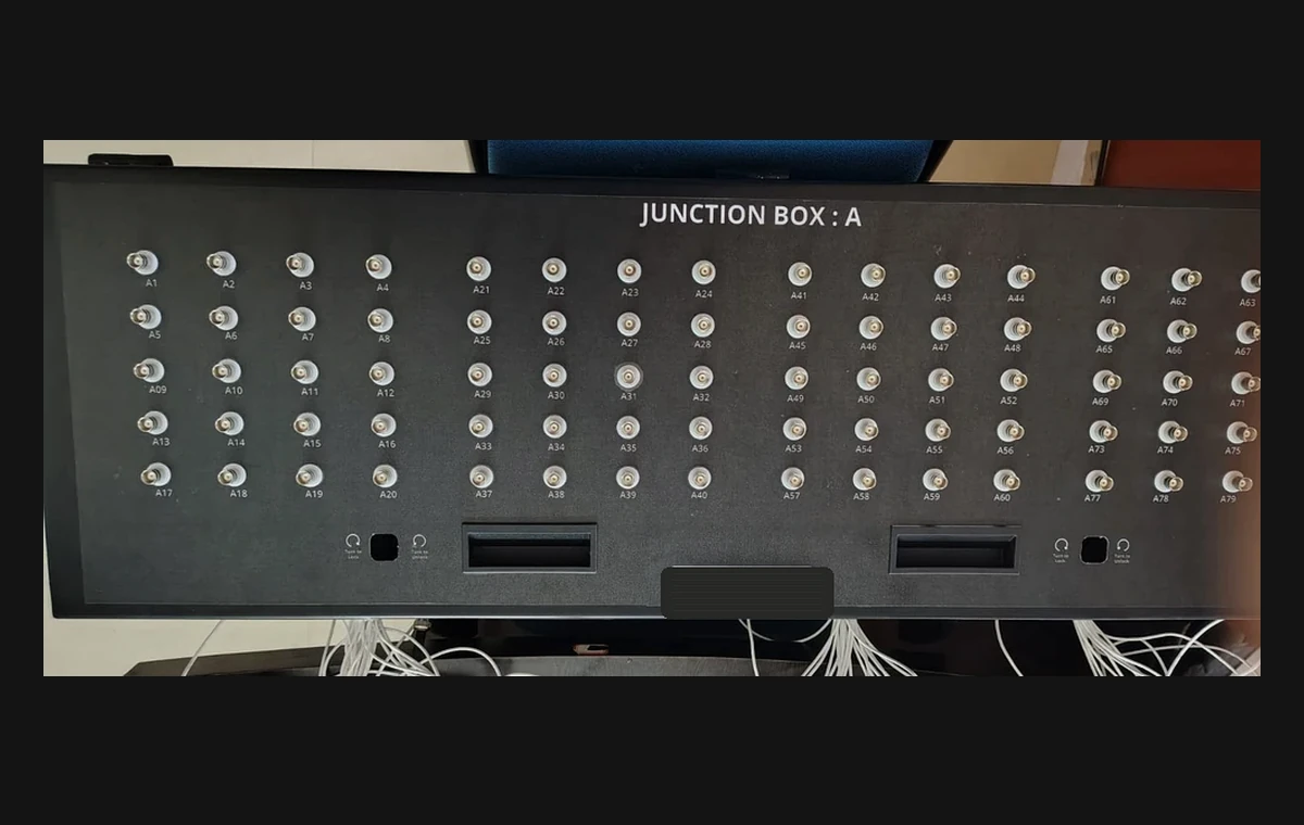
PhonoVibe HD — 16-Channel IEPE DAQ
Multi-point simultaneous acquisition, so a dataset carries phase relationships and not just single-channel levels.
- Channels
- 16

To-Learn Vibe — Vibration Simulation Training Software
Generate signal cases to stress a pipeline before committing rig time to them.
From the TIERA store
The kit for this job
What we would actually put in front of someone doing the measurement this post describes — not the whole catalogue.
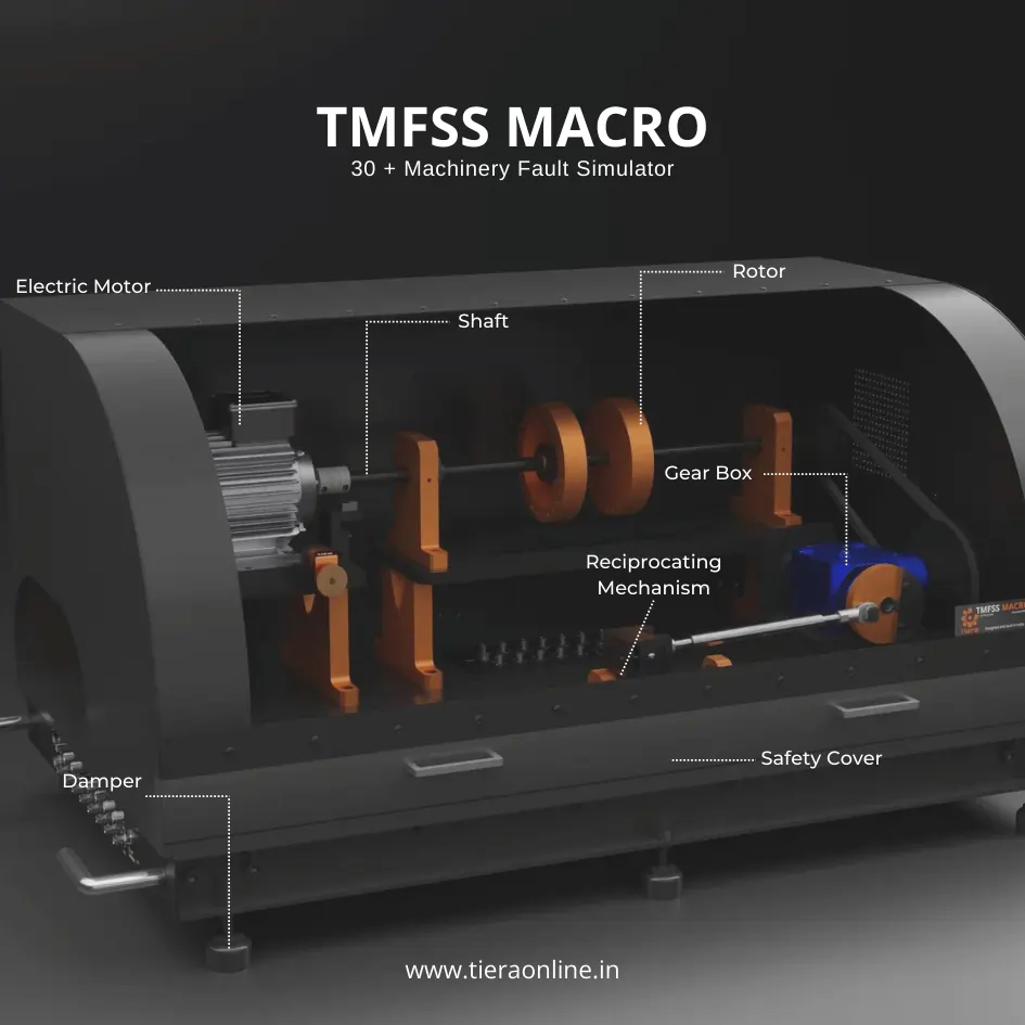 Machinery Fault Signature SimulatorTiera’s Machine Fault Simulator (TMFSS) is a valuable tool for industries and researchers, simulating over 30 real-world faults such as: Bearing faults: outer race defects, inner race defects, cage defects. Motor faults: stator faults, rotor faults, electrical unbalance. Gearbox faults: gear wear, misalignment, gear tooth damage. Etc..₹13,53,600View →
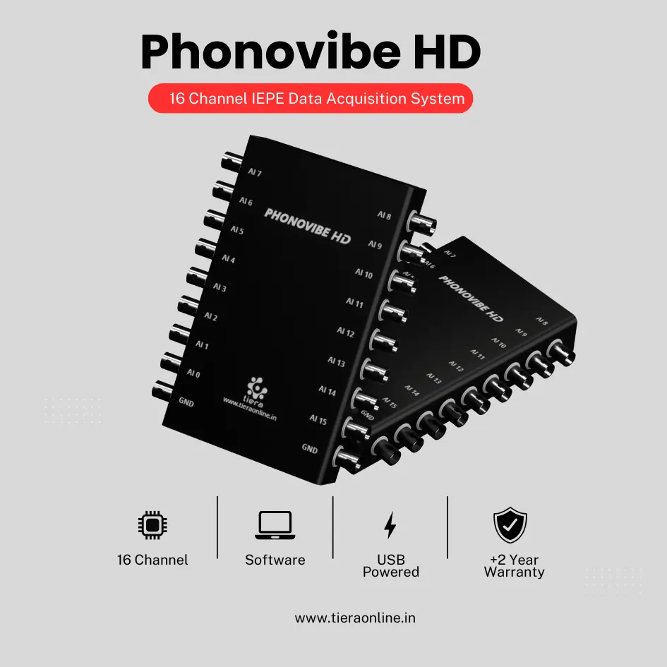 16 Channel IEPE Data Acquisition System-Phonovibe HDSixteen-Channel Data Acquisition System Plug & Play USB Powered Compatible with accelerometers, microphones, hammers, and other IEPE sensors T-VIB Software for time waveforms, frequency spectra, vibration levels, FRFs, and octave measurements Base version includes Time and Spectrum with TSAP 201 post-processor Explore additional modules with T-VIB Software₹7,20,000View →
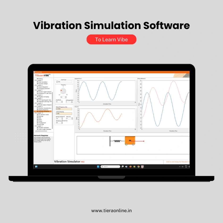 To Learn Vibe -Vibration Simulation Software Basic (Yearly Subscription)For comprehensive vibration analysis training, start with our To Learn Vibe software. Covering everything from basic to advanced vibration concepts, this software is designed to kickstart your career and enhance your expertise. Perfect for mastering fundamental and advanced vibration analysis, To Learn Vibe equips you with the knowledge and skills needed to excel in the field of vibration engineering.₹34,560View →
Use cases
Where this shows up in the field
A dataset your result survives contact with.
ML teams come to us when a model that scored 99% in the notebook fell over on the second machine. The fix is almost never the architecture — it is the data and the split.
TMFSS gives you multiple configurations, graded severities and repeatable labels, which is what makes a group-split evaluation possible in the first place.
- TMFSS for labelled, severity-graded faults across configurations
- PhonoVibe HD for multi-point simultaneous acquisition
- Guidance on splitting, baselines and reporting that survives review
Where this sits on the TIERA learning ladder.
The theory behind this article is covered free, in full, by the TIERA 101 primers: AI Condition Monitoring 101, Signal Processing 101. They are self-paced, interactive, and end in an exam and a certificate.
The primer covers what AI can and cannot do in condition monitoring. Group-aware evaluation, leakage detection and honest prognostics reporting are the Cat III/IV material.
TIERA 101 is a free introductory primer, not an accredited ISO certification, and its hours do not count towards the formal training ISO 18436 requires.