Heavy Spot vs High Spot: Why the Vibration Does Not Point Where the Weight Is
The heavy spot is where the unbalance mass sits; the high spot is where the orbit peaks — what the sensor sees. Between them is a phase lag that swings from 0° to 180° as speed crosses the critical. Understanding that lag explains rotor inversion, why a balance job can look wrong at another speed, and why the correction angle is measured, never assumed.
Two spots, one rotor — and they are not the same place
- The heavy spot is a place on the rotor; the high spot is a response — and your instrument only ever sees the second one.
- They are separated by the phase lag between the rotating unbalance force and the rotor's displacement.
- That lag is not a constant: it runs from roughly zero to roughly 180 degrees, with the crossover at the critical speed.
Anyone who has balanced a few rotors has met the moment when the numbers stop making sense. The analyser reports the 1× vibration peaking at, say, 118 degrees past the tach mark — so surely the excess mass sits somewhere near 118 degrees, and the correction weight goes opposite it. Except the solver puts the weight somewhere else entirely, the machine smooths out, and you are left wondering what the phase reading actually pointed at. The answer is that there are two different spots on that rotor, and the instrument only ever sees one of them.
The heavy spot is a physical place: the angular position where the unbalance mass actually sits — a casting void's opposite side, a lump of weld, an erosion-thinned blade's opposite number. The high spot is a response: the direction in which the shaft's whirl orbit reaches its peak, which is what a probe or accelerometer on the bearing reports. The two rotate together, locked to the shaft, but they are separated by an angle — the phase lag between the rotating unbalance force and the rotor's displacement response. That lag is not a nuisance constant. It changes with speed, from roughly zero to roughly 180 degrees, and the crossover happens at the critical speed. Almost every balancing confusion traces back to treating these two spots as one.
The clean theory: one mode, one formula
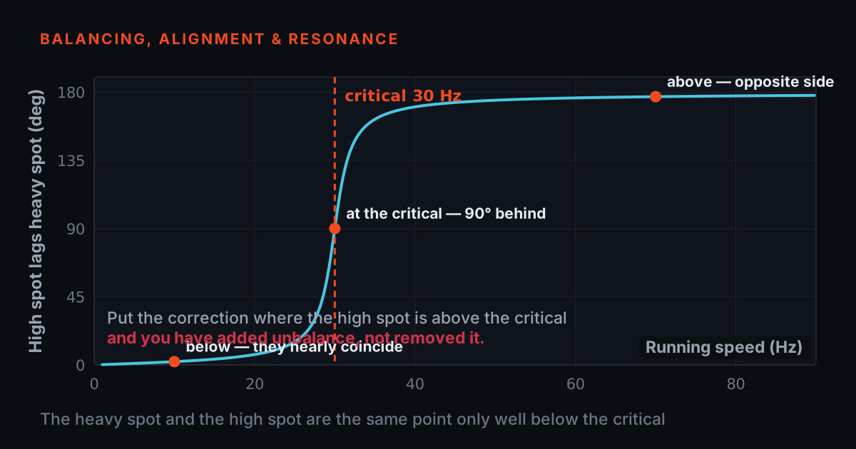
Strip the problem to its textbook skeleton — a single disc on a flexible shaft, one natural frequency, viscous damping — and the whole story is one formula. Call the speed ratio r = running speed ÷ critical speed and the damping ratio ζ. The displacement response lags the rotating unbalance force by δ = atan2(2ζr, 1 − r²): near 0° well below the critical, exactly 90° at r = 1, approaching 180° far above it. The whirl radius, in units of the rotor's mass eccentricity, is r² ÷ √((1 − r²)² + (2ζr)²) — small at low speed, peaking near the critical, and settling toward exactly 1 at high speed. Those two curves are the entire physics of this post.
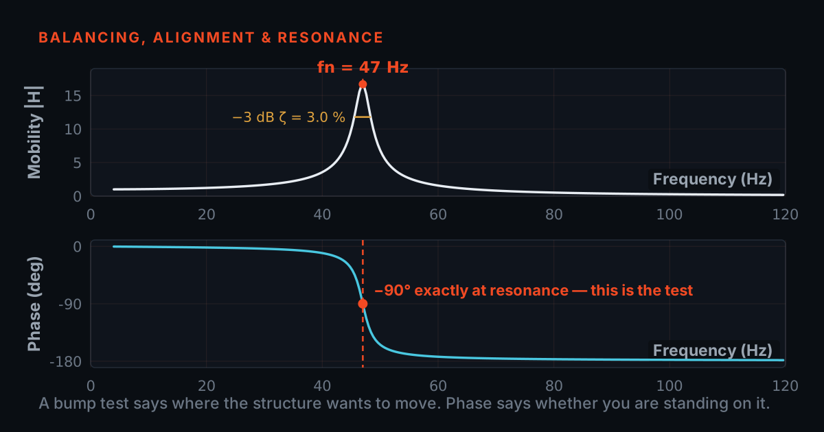
The 90° point deserves a physical explanation rather than a formula. Below the critical, the shaft's stiffness dominates: push, and it deflects essentially in step with the push, like leaning on a spring. At the critical, the spring force and the inertia force cancel each other — that cancellation is what resonance is — and the only thing left resisting the unbalance force is damping, which acts on velocity, not displacement. Velocity peaks a quarter cycle before displacement does, so for the force to be feeding the damper, the displacement must run a quarter turn behind the force: 90 degrees. Damping never moves that crossing — every curve in the figure passes through 90° at exactly r = 1 — it only decides how abruptly the phase turns around it. At ζ = 5% the turn is a cliff; at 25% it is a long ramp spread over half an octave of speed.
Below, at, above: the rotor inversion
- Below the critical the two spots very nearly coincide, which is why low-speed intuition — "it vibrates where the weight is" — genuinely works there.
- Above the critical the rotor inverts: it spins about its mass centre, and the residual whirl of the geometric centre settles at exactly the mass eccentricity and stops growing with speed.
- That is why large turbomachinery is deliberately run supercritical — and why the vibration vector up there points away from the mass you are trying to counteract.
Walk a rotor up through those three regimes and something remarkable happens. Below the critical (spring-controlled), the high spot sits nearly on top of the heavy spot: the shaft bows out on the same side as the mass, and low-speed intuition — 'it vibrates where the weight is' — is genuinely correct. At the critical (damping-controlled), the high spot has fallen a quarter turn behind: the orbit peaks 90 degrees after the heavy spot passes the probe. Well above the critical (mass-controlled), the lag approaches 180 degrees and the geometry quietly turns inside out: the shaft's geometric centre now whirls on the opposite side from the mass, and since the whirl radius has settled at exactly one eccentricity, the mass centre ends up sitting almost still on the bearing centreline. The rotor is no longer spinning about its geometric centre — it is spinning about its mass centre, with the geometry orbiting around it.
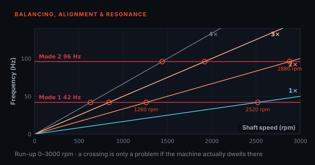
This is the rotor inversion, sometimes called critical speed inversion or self-centring, and it is not a mathematical curiosity — it is why large turbomachinery is deliberately run supercritical. Above the critical, the rotor finds the axis it always wanted: the residual whirl of the geometric centre equals the mass eccentricity and gets no worse with speed, so a supercritical machine can run smoother than the same machine fighting its unbalance just below the critical. For a balancer, though, inversion carries a sting: the vibration vector your instrument reports now points away from the mass you are trying to counteract. If you have already driven a virtual machine through its critical on the amplitude side in our Campbell explorer at /blog/campbell-resonance-explorer, this is the same run-up seen from the phase side.
Drag the speed and watch the spots separate
The simulator below runs the honest single-mode mathematics live — lag from atan2(2ζr, 1 − r²), whirl radius from the unbalance response, nothing faked. The rotor face on the left shows the heavy spot (solid), the high spot (hollow) and the mass centre (small dot), with the whirl orbit exaggerated so you can see it; the curves on the right show where the current speed sits on the amplitude and phase characteristics.
One convention, stated once and used in every figure on this page and in the solver at /blog/balancing-solver-simulator: angles run from the tach mark, positive counter-clockwise viewed from the measurement end, and the shaft here turns counter-clockwise. δ is a lag, so the high spot always sits δ degrees BEHIND the heavy spot in the direction of rotation — it reaches the probe δ degrees of shaft rotation later. Flip the rotation and the picture mirrors; the lag is still behind.
Three experiments are worth your time. First, set damping to 5% and drag the speed ratio slowly from 0.6 to 1.4: watch how little the high spot moves until about r = 0.9, then how violently it swings through a quarter turn — that abruptness is why phase readings taken near a critical are so twitchy run to run. Second, park at r = 1.0 and sweep the damping slider: the lag stays pinned at 90° while everything around it changes — the crossing is a property of resonance itself, not of the damping. Third, jump to r = 2.5 and watch the mass centre: it settles onto the bearing centreline crosshair while the geometry whirls around it. That is inversion, happening in front of you.
Why balancing software asks you to measure phase, never to reason it out
- "Weight opposite the vibration" is not a simplification above the critical — it is the exact wrong answer, placing the correction on top of the unbalance.
- The influence-coefficient method never asks where the mass is; it measures the machine's response to a known weight, and that vector absorbs the phase lag along with sensor, integrator, filter and tach-edge shifts.
- That is why nothing in the procedure needs the critical speed or the damping ratio to be known.
Here is the trap in full. A fitter who knows the machine runs below its critical can get away with the folk rule 'put the weight opposite where it vibrates most', because down there the high spot and the heavy spot roughly coincide. Apply the same rule to a machine running above its critical and the logic inverts with the rotor: the high spot is already opposite the heavy spot, so 'opposite the high spot' places the correction weight on top of the unbalance mass — and the next run is worse than the first. Between those extremes, near the critical, the honest answer is 'somewhere in a 180-degree range depending on ζ and exactly where the critical sits' — and you know neither number to the precision a correction angle needs.
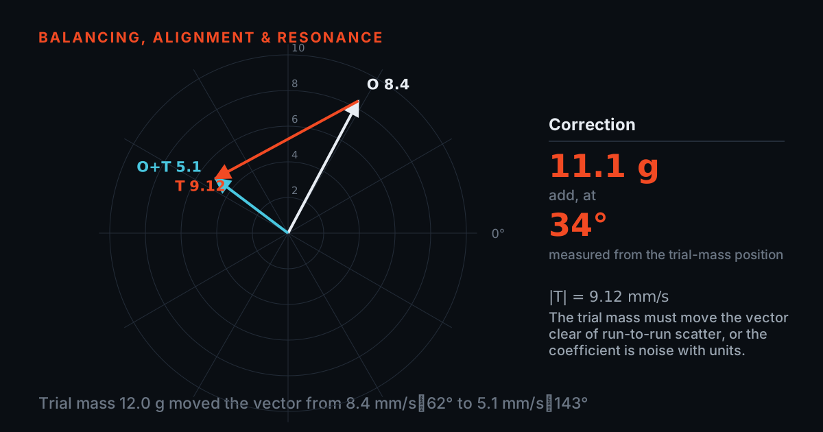
This is precisely why serious balancing procedure never asks where the weight must be. The influence-coefficient method — the reference-run, trial-weight, correction sequence walked through at /blog/field-balancing-trial-weights — measures the machine's actual response to a known weight, and that measured vector silently absorbs the phase lag, wherever the machine sits relative to its criticals, along with every other phase shift in the chain: the sensor's own response, integrator phase, filter delays, tach-edge offsets. Nothing is assumed; everything is calibrated in one trial run. It also explains the rule that every balancing manual states and this post can now justify: do the job at operating speed, and never mix readings taken at different speeds. An influence coefficient is a property of the machine at one speed. Take the reference run at 1,000 RPM and the trial run at 1,500 with a critical in between, and the two vectors you are subtracting were measured in different physical regimes — the arithmetic will still produce a confident, wrong answer. If you want to feel how the vector arithmetic behaves when the readings are consistent, the solver at /blog/balancing-solver-simulator lets you practise exactly that — notice it never asks for the natural frequency, because the trial weight measures around it.
A representative case, not a specific customer
The numbers below are typical of this class of problem, not a record of any customer or machine. An induced-draft fan is balanced during commissioning with the VFD capped at 900 RPM for safety. The job goes textbook: 1× drops from 8.2 mm/s to 1.1 mm/s, phase steady, report filed. Weeks later the cap is lifted and the fan runs at its 1,480 RPM duty point — and reads 2.1 mm/s at 1×, with the phase some 130 degrees away from anything in the balancing report. The crew's first theory is that a weight has shifted. It has not: the rotor-support system has a critical near 1,100 RPM, so the readings at 900 and at 1,480 sit on opposite sides of the phase turn. The residual unbalance that was acceptably placed for the subcritical regime is being read through a completely different lag at duty speed, and at nearly twice the level: velocity rises with speed, and the response term r² ÷ √((1 − r²)² + (2ζr)²) is a little larger on the far side of the critical than it was on the near side.
The fix is undramatic: rerun the whole procedure — reference, trial, correction, verification — at 1,480 RPM, treating the 900 RPM data as belonging to a different machine, because dynamically it does. Final reading 1.3 mm/s at duty speed. The lesson generalises: a balance state is only defined at the speed where it was measured, and a machine with a critical inside its operating range may need the acceptance argument stated at more than one speed. Nothing here required abandoning the earlier work as 'wrong' — it was correct at 900 RPM, and meaningless at 1,480.
What the clean theory hides — and where to learn the rest
Everything above leaned on an idealised model, and honesty requires listing what it hid. Real rotors have several modes, and each one takes its own 180-degree phase turn — cross two criticals on the way to duty speed and the cumulative lag heads for 360, with plateaus and partial recoveries in between, as in the figure. Real damping is rarely known better than 'somewhere between 2% and 10%', so the width of the phase transition is uncertain even when the critical itself is well located. Real supports are asymmetric — horizontal stiffness usually differs from vertical — which splits each critical into a pair and makes the orbit elliptical, so 'the' high spot is itself a simplification: the peak of an ellipse, in a direction that need not line up with either measurement axis. Add gyroscopic effects, which move the natural frequencies with speed, and foundation dynamics, and '90 degrees at resonance' is properly read as the clean-theory anchor point, not a promise about your fan. All of which is one more argument for the same conclusion: measure the response, never derive it.
If you want the supporting theory at a gentler pace, the free primers at 101.tieraonline.in cover it from both ends — Balancing & Alignment 101 for the balancing procedure and phase conventions, Modal & Resonance 101 for natural frequencies, damping and mode shapes. TIERA 101 is a free primer, not an accredited ISO certification. For formal, examined analyst training there is the TCAT programme on our services page at /services, with proctored examinations at exams.tieraonline.in.
TIERA instruments that do this work.
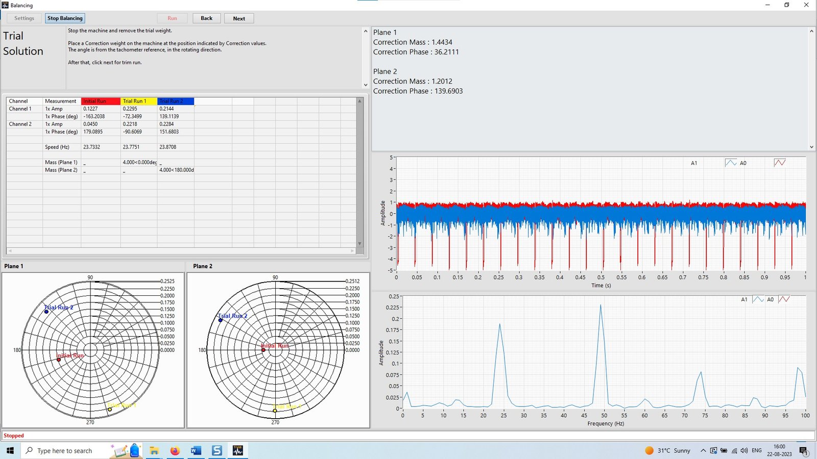
TVIB TB 210 — Two-Plane Field Balancing Module
Implements exactly what this post argues for: the correction angle comes from a measured phase against a tach or laser reference, so the speed-dependent lag is absorbed by the trial run instead of guessed.
- Balancing planes
- Single-plane and two-plane
- Phase reference
- Tachometer or optical laser trigger
- Output
- Correction weight, correction angle, balancing report
- Compatible DAQ
- PhonoVibe series; NI 9234 / 4431; Modal Shop 485B39; Sinus Apollo; DT9837
- Licence type
- Perpetual; 2 years free updates

PhonoVibe Series — Sound & Vibration DAQ
Phase is a timing measurement: simultaneous sampling on every input puts all channels on one clock, so the lag you read belongs to the rotor, not the instrument chain.
- ADC resolution
- 24-bit
- Sampling
- Simultaneous on every input
- Sensor power
- 24 V, 4 mA constant current (IEPE / ICP / CCLD)
- TEDS
- Supported
- Calibration
- Factory calibration certificate, 1-year validity

TMFSS — Machinery Fault Signature Simulator
The rig for seeing the inversion yourself: controlled unbalance, VFD speed control and a built-in tach let you walk a rotor from sub-critical to super-critical and watch the high spot fall behind the heavy spot.
- Faults (Macro)
- 30+ base kit, extensible with add-on kits
- Speed control
- VFD with WiFi software
- Tachometer
- Built-in, analog output
- Foundation
- Solid rigid base
- Warranty
- 1 year; AMC available
From the TIERA store
The kit for this job
What we would actually put in front of someone doing the measurement this post describes — not the whole catalogue.
 TB 208 – Balancer (Phonovibe Q)Use Cases Balancing Rotating Machineries₹69,120View →
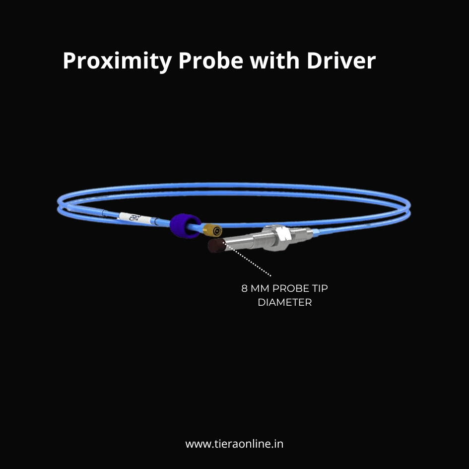 Proximity Probe with DriverPROXIMITY PROBE, 8 MM PROBE TIP DIAMETER, WITH 3/8-24 OR M10X1 CASE THREAD Measure shaft vibration and displacement on machinery with fluid film bearings. Durable PPS over-molded probe tips withstand harsh conditions when monitoring critical machinery such as turbines and compressors. Complete hardware system is compatible with all standard condition monitoring software EDDY CURRENT DRIVER COMPATIBLE WITH 8 MM PROXIMITY PROBE SYSTEMS, VOLTAGE OUTPUT API Standard 670 specified format Isolated voltage output standard at BNC and terminal block Vout and Com Upgraded to include SecureLock connector₹88,000View →
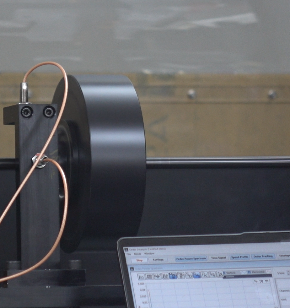 Resonance Simulation KitResonance Faults Addon Kit for the TMFSS Macro simulates resonance-related faults in industrial machines₹1,87,500View →
Use cases
Where this shows up in the field
Stop guessing the lag — measure it.
The whole argument of this post lands on one practical requirement: the correction angle must come from a measured phase, referenced to a physical mark on the shaft, taken at the speed the machine actually runs. That is exactly what the TVIB TB 210 balancing module does — tachometer or optical laser phase reference, guided reference and trial runs, influence coefficients solved for single-plane and two-plane jobs, and the correction weight and angle stated directly, with the residual checked against ISO 1940 grade limits and a report for the maintenance file. The phase lag never becomes your problem, because the trial run measures it.
The measurement chain underneath matters just as much: a phase reading is only as good as the timing between channels. PhonoVibe DAQs sample every input simultaneously — 24-bit, IEPE sensor power, TEDS recognition — so the timing relationship between simultaneously-acquired channels is preserved, not reconstructed; the phase reference itself comes in through TB 210, from a tachometer or laser. And if you want to see the inversion with your own eyes rather than trust a blog post, the TMFSS simulator is built for exactly that experiment: controlled unbalance, VFD speed control and a built-in tachometer, so you can walk a rotor up through its critical on a bench and watch the phase turn — with nothing at stake.
- TB 210: guided single- and two-plane balancing with tach or laser phase reference — the lag is measured, never assumed
- PhonoVibe: simultaneous 24-bit sampling keeps vibration and tach channels phase-true
- TMFSS: run the sub-critical → critical → super-critical experiment yourself, with controlled unbalance and a built-in tach
- 14-day fully-unlocked TVIB trial available if you want to explore the workflow first
Where this sits on the TIERA learning ladder.
The theory behind this article is covered free, in full, by the TIERA 101 primers: Balancing & Alignment 101, Modal & Resonance 101. They are self-paced, interactive, and end in an exam and a certificate.
TCAT adds structured, examined analyst training with proctored exams — the free primers give you the phase-lag theory; TCAT verifies you can apply it on a live machine.
TIERA 101 is a free introductory primer, not an accredited ISO certification, and its hours do not count towards the formal training ISO 18436 requires.