Solve a Single-Plane Balance Yourself: A Live Influence-Coefficient Solver
Enter a reference run, a trial weight and a trial run, then drag the weight around the rotor and watch the correction mass and angle update live. The arithmetic behind every field balance, running in your browser.
This time, you do the solving
- You give a balancing instrument three measured things and it returns two: a correction mass and an angle.
- The model is linear, single-plane and constant-speed — doubling a weight doubles its effect, one correction plane is enough, and every run happens at the same RPM.
- The influence coefficient is only valid at the speed where it was measured, which is what pins the whole procedure to one RPM.
Our field-balancing explainer walks the whole job — confirming the fault is really unbalance, sizing and fastening the trial weight, reading the result against an ISO 21940 grade. What it could not do on a static page is hand you the rotor. This post does: further down is a live influence-coefficient solver. You give it the three things a balancing instrument measures, and it gives you the two things a balancing instrument reports — a correction mass and an angle.
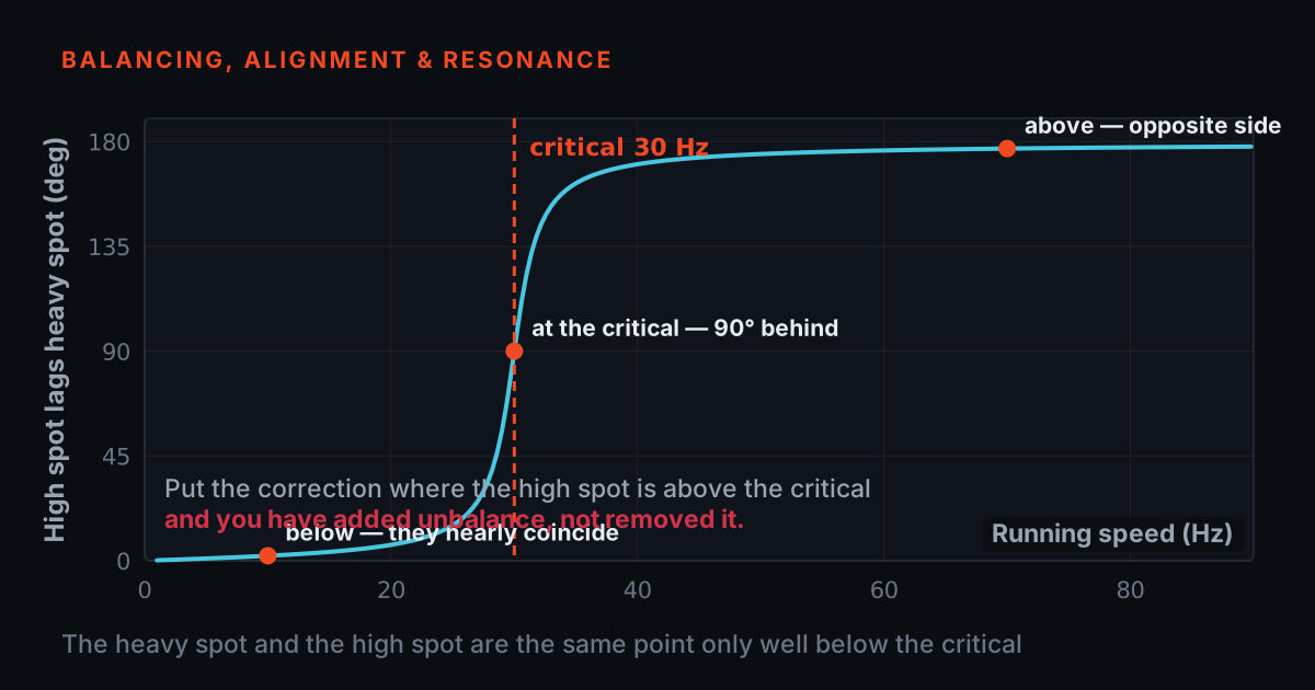
The model is stated up front so there is no mystery: a linear, single-plane rotor at constant speed. Linear means doubling a weight doubles its effect; single-plane means one correction plane is enough (thin discs, fans, flywheels); constant speed means every run happens at the same RPM, because the rotor's response to unbalance — the influence coefficient — is only valid at the speed where it was measured. Inside that box, the whole job is three vectors in and one weight out.
Pick an angle convention and never let go
Every number in this job is an amplitude plus an angle, so the convention has to be nailed down before anything else. The solver's is simple: angles are measured in degrees from the once-per-revolution reference mark — the strip of reflective tape the tachometer sees — and positive angles run counter-clockwise, viewed from the measurement end. Phase readings and weight positions use the same zero and the same direction. That is the entire convention.
It matters because most 'the maths is wrong' arguments in balancing are convention bugs, not arithmetic. Instruments differ in whether displayed phase leads or lags, and rotors get viewed from either end. Whichever convention your instrument uses, the discipline is identical: one zero, one positive direction, applied to every phase reading and every weight angle, written on the job sheet. Flip either one halfway through and the correction lands mirror-imaged — confidently, and wrongly.
The solver: three readings in, one correction out
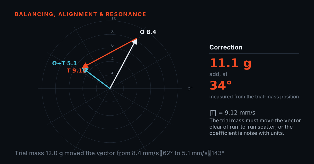
Enter the reference run O (amplitude and phase), the trial weight (mass and angle), and the trial run O+T. The plot draws O and O+T from the centre, joins their tips with the derived effect vector T, and marks −O — the direction the correction's effect must push. The panel below the plot reports T, the influence coefficient H, the correction mass and angle with the trial weight removed, and the predicted residual once the correction is rounded to something you could actually fit.
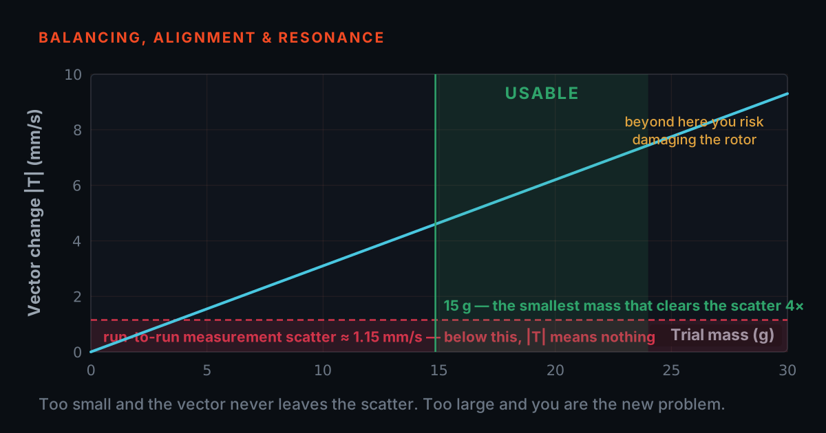
Two ways to play. Drag the orange dot around the rim: it is the trial weight, and out of the box the trial-run reading is simulated live from a hidden rotor, so the reading and the solution move as the weight does. Or press Randomise a job for a fresh rotor with a different hidden influence coefficient, and practise reading the answer. Type your own numbers into the O+T boxes at any point and the solver switches to trusting your readings instead. If the trial effect is too small to trust, it will tell you — the same 'make the trial matter' rule the field job has.
O — reference run O+T — trial run T — trial-weight effect −O — where the correction must push trial weight (drag it) solved correction angle
Model: a linear, single-plane rotor at constant speed — every run at the same speed, same sensor, same tacho mark. Angles are degrees from the reference mark, positive counter-clockwise viewed from the measurement end. The correction assumes the trial weight is removed; the residual assumes it is fitted to the nearest 0.5 g and 1°. A real job still ends with a verification run.
What the solver is doing underneath
- Where you choose to hang the trial weight cannot change where the machine's unbalance is — the rotation of ∠φ and the rotation of the measured effect cancel.
- So a solved correction that stands still while you drag the trial weight is the answer being right for the right reason.
- The predicted residual only accounts for rounding the correction to a fittable mass and angle; the verification run is what settles it.
Each reading is a complex number: amplitude at an angle. Step one is complex subtraction, T = (O+T) − O, tip to tip on the plot — the trial weight's own effect, isolated. Step two divides that effect by the trial weight as a vector, H = T ÷ (m∠φ), giving the influence coefficient: what one gram at zero degrees would do to this rotor, in these bearings, at this speed. Step three is the payoff, W = −O ÷ H: the mass and angle whose predicted effect lands exactly opposite the original reading. Complex division is just dividing magnitudes and subtracting angles — the polar chart methods of the paper era were this same arithmetic done graphically.
The drag behaviour now explains itself. While the hidden rotor is live, moving the trial weight rotates the ∠φ term AND rotates the measured T with it by exactly the same angle, so the two rotations cancel in H = T ÷ (m∠φ) and the solved correction stands still. That is the physical answer: where you choose to hang the trial weight cannot change where the machine's unbalance is. The correction only swings if you rotate ∠φ while holding the readings fixed — which is a mis-recorded weight angle, not a different rotor, and is the failure the next section makes you commit on purpose. And note what the predicted residual is: the model grading its own homework. It only reflects rounding the correction to a fittable mass and angle; real rotors add nonlinearity, speed drift and measurement noise, which is why the field procedure ends with a verification run, not a prediction.
A representative practice job
A representative job, not a specific customer: a direct-coupled blower at 2,950 RPM reads 8.0 mm/s at 40° on the reference run. A 25-gram trial weight bolted at the 0° mark moves the reading to 9.3 mm/s at 358.3° — the amplitude went up, which is fine; the vector moved by over 6 mm/s, and that is what solves the coefficient. Those are the solver's pre-loaded defaults, so you can check its working: the effect T comes out near 6.3 mm/s at 300°, the influence is about 0.25 mm/s per gram, and the correction lands at roughly 32 grams at 280° with the trial weight removed.
The predicted residual is under 0.1 mm/s — and on a real machine you would trust that exactly as far as the verification run confirms it. Now do what the page version of this job cannot: type 90 into the trial-weight angle, then re-type the original trial run — 9.3 mm/s at 358.3° — back into the O+T boxes, because typing there detaches the hidden rotor and makes the solver trust your readings as recorded. The correction swings from 280° to 10°, by exactly the 90° you mis-attributed. Same vectors, different attribution, different answer — a five-second demonstration of why the weight angle gets written down before the run, not remembered afterwards.
Three rules the simulator cannot teach you
The solver waives nothing that matters at the machine. Same speed, every run — reference, trial, correction, verification — because the influence coefficient dies the moment the speed changes. Trial weight off, or on, never halfway: the correction differs for each case, so decide before fitting, tag the rotor, and write it down. And fasten every weight so it cannot fly off — centrifugal force grows with speed squared, and a modest trial mass at radius pulls outward with tens of kilograms of force at ordinary machine speeds. Bolt it, clamp it, or weld it; never tape it; stand clear of the rotor's plane during run-up.
If the vector arithmetic felt quick, the free primers at 101.tieraonline.in take it at beginner pace — the Balancing & Alignment 101 course covers phase, conventions and the influence-coefficient method from first principles. TIERA 101 is a free primer, not an accredited ISO certification. For formal, examined analyst training there is the TCAT programme on our services page, with proctored examinations at exams.tieraonline.in.
- Run reference, trial, correction and verification all at the same speed.
- Decide before fitting whether the trial weight stays on or comes off, tag the rotor, and write it down.
- Write the trial weight's angle on the job sheet before the run.
- Bolt, clamp or weld every weight so it cannot leave the rotor.
- Finish with a verification run rather than the solver's predicted residual.
- Do not subtract two runs measured at different speeds — the influence coefficient dies when the speed changes.
- Do not leave the trial weight half-decided; the correction differs for each case.
- Do not reconstruct a weight angle from memory after the run.
- Do not tape a weight on — centrifugal force grows with speed squared and reaches tens of kilograms at ordinary machine speeds.
- Do not stand in the rotor's plane during run-up.
TIERA instruments that do this work.
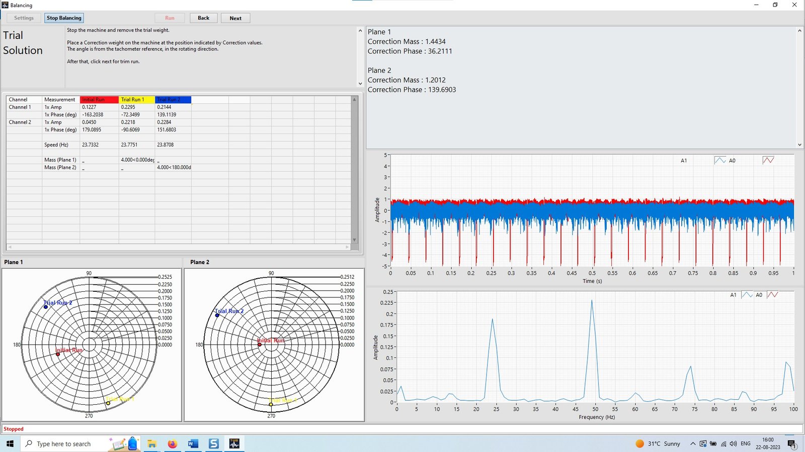
TVIB TB 210 — Two-Plane Field Balancing Module
The guided version of this exact arithmetic: prompted trial-weight runs, automatic correction weight and angle, and a residual check against ISO 1940 grade limits.
- Balancing planes
- Single-plane and two-plane
- Phase reference
- Tachometer or optical laser trigger
- Output
- Correction weight, correction angle, balancing report
- Host software
- TVIB TSAP 201 base module required
- Licence
- Perpetual; 2 years free updates

PhonoVibe Series — Sound & Vibration DAQ
The recommended DAQ for running TB 210 in the field — 24-bit, USB bus-powered from the laptop, with IEPE sensor power for the accelerometer on the bearing housing.
- ADC resolution
- 24-bit
- Channels
- 2 / 4 / 8 / 16 (D, Q, O, HD)
- Sensor power
- 24 V, 4 mA constant current (IEPE/ICP/CCLD)
- Connectivity
- USB, plug-and-play (Windows 10 / 11)
- Calibration
- Factory calibration certificate, 1-year validity

TMFSS — Machinery Fault Signature Simulator
Practise the full loop beyond the browser: set a known, repeatable unbalance on a benchtop rotor, balance it out, and get the trial weight deliberately wrong with nothing at stake.
- Fault library (Macro)
- 30+ faults in base kit, including unbalance and misalignment
- Speed control
- VFD with WiFi software
- Tachometer
- Built-in, analog output
- Foundation
- Solid rigid base — repeatable signatures across sessions
From the TIERA store
The kit for this job
What we would actually put in front of someone doing the measurement this post describes — not the whole catalogue.
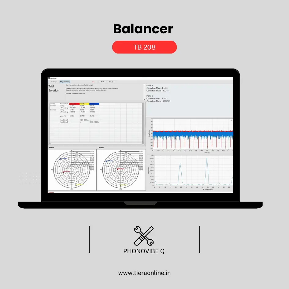 TB 208 – Balancer (Phonovibe Q)Use Cases Balancing Rotating Machineries₹69,120View →
- Balancing Kit — Phonovibe QField balancing, hardware and software together — Phonovibe Q DAQ, the TB 208 balancer application, an accelerometer and cable.Request priceView →
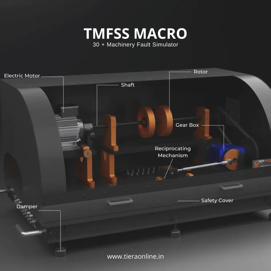 Machinery Fault Signature SimulatorTiera’s Machine Fault Simulator (TMFSS) is a valuable tool for industries and researchers, simulating over 30 real-world faults such as: Bearing faults: outer race defects, inner race defects, cage defects. Motor faults: stator faults, rotor faults, electrical unbalance. Gearbox faults: gear wear, misalignment, gear tooth damage. And more.₹13,53,600View →
Use cases
Where this shows up in the field
When the rotor is real, take the guided version
The solver on this page is the arithmetic; a field job also needs the measurement done right. The TVIB TB 210 balancing module runs this exact sequence guided step by step — tachometer or laser phase reference, prompted trial-weight runs, automatic correction weight and angle for single-plane and two-plane rotors, and a balancing report for the maintenance file. It runs on any PhonoVibe DAQ; the two-channel PhonoVibe D, 24-bit with IEPE sensor power and USB-powered from the laptop, makes a natural field kit.
To practise beyond a browser, the TMFSS simulator generates controlled, repeatable unbalance on a benchtop — set a known heavy spot, balance it out, get the trial weight deliberately wrong, and see the consequences with nothing at stake.
- TB 210: guided single-plane and two-plane balancing with phase correction and a report
- PhonoVibe DAQ: 24-bit simultaneous capture — the recommended DAQ for running TB 210 in the field
- TMFSS: repeatable, known unbalance for practising the full loop
Where this sits on the TIERA learning ladder.
The theory behind this article is covered free, in full, by the TIERA 101 primers: Balancing & Alignment 101. They are self-paced, interactive, and end in an exam and a certificate.
TCAT adds formal, examined training with proctored exams — the free primer teaches the vectors; TCAT verifies you can run the job.
TIERA 101 is a free introductory primer, not an accredited ISO certification, and its hours do not count towards the formal training ISO 18436 requires.