Build the Spectrum Yourself: What Unbalance, Misalignment and Looseness Actually Look Like
An interactive mini-explainer: assemble a machine's vibration from its parts — 1x, 2x, a harmonic comb — and watch the time waveform and spectrum change live. Learn the three classic signatures by driving them.
The waveform is a sum. The spectrum is the receipt.
An accelerometer bolted to a bearing housing measures exactly one thing: how the housing moves. It does not know why. A heavy spot on the rotor pushes on it once per revolution. A misaligned coupling loads it twice per revolution. A loose hold-down bolt lets the foot lift and slap back down, adding a sharp impact on top of everything else. All of it lands in the same signal, added together into one wiggly line — the time waveform.
The FFT is the un-mixer. Every periodic ingredient in the waveform gets its own vertical line in the spectrum, at its own frequency, with a height equal to its contribution. Reading spectra is pattern recognition on those lines — and the fastest way to learn the patterns is to run the machine backwards: start from the ingredients, mix them yourself, and watch the waveform and spectrum form in front of you. That is what the simulator below does.
Drive it yourself: mix a fault, read the verdict
Four sliders. The 1x slider is the heavy spot — a smooth sinusoid at running speed, the signature of unbalance. The 2x slider is what a misaligned coupling adds at twice running speed. The harmonics slider pours in a decaying comb from 3x to 8x — the fingerprint of looseness, because a once-per-revolution impact cannot be described by one sine wave; it takes a whole family of them. The speed slider moves everything along the frequency axis in Hz while the pattern of orders (1x, 2x, 3x...) stays put — which is exactly why analysts think in orders of running speed, not raw hertz.
Nothing here is a canned picture. The waveform is genuinely the sum of the sinusoids you dial in, and the spectrum is computed from that waveform by a discrete Fourier transform — change a slider and both plots are recalculated. Try three experiments: push 1x up alone and watch a single clean line grow; add 2x until the verdict line changes its mind; then drag the harmonics slider up and watch the smooth waveform turn spiky as the comb marches across the spectrum.
Unbalance: one heavy spot, one lonely line
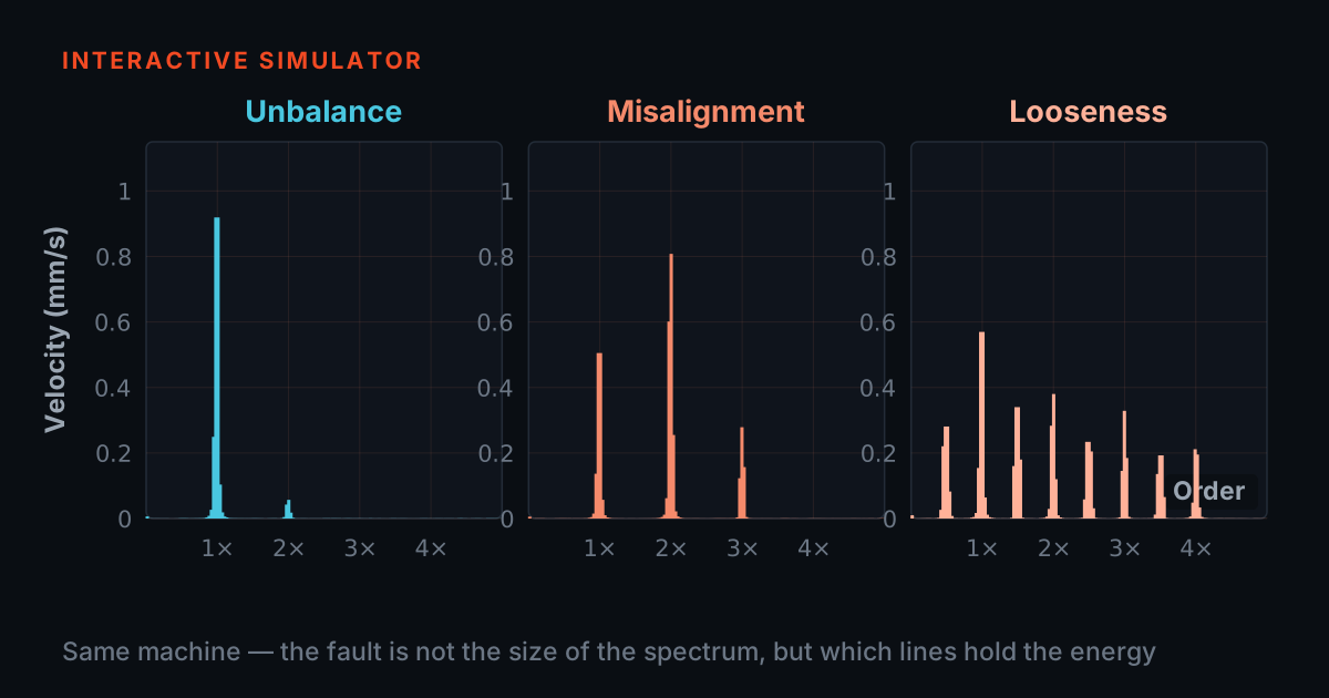
- The diagnosis is in what is not there: a dominant 1x with quiet 2x, 3x and beyond. Broadband growth across the spectrum is not unbalance.
- Selectivity is the tell. Step a trial mass up and only the 1x line climbs while its neighbours stay put — push the 1x slider alone in the simulator and you get the same picture.
- A bent shaft and an eccentric rotor also raise 1x, so phase and the speed-squared test are what separate them in the field.
A heavy spot on a rotor produces a centrifugal force that rotates with the shaft — the bearing feels one push per revolution, so the vibration is a clean sinusoid at exactly 1x running speed, strongest in the radial direction. The force grows with the square of speed: double the RPM and the unbalance force quadruples, which is why a rotor that is acceptable at 1,500 RPM can be rough at 3,000.
The discipline is in what is not there. A dominant 1x with quiet 2x, 3x and beyond is the unbalance picture; broadband growth is not unbalance, and a bent shaft or an eccentric rotor can also raise 1x, so phase and the speed-squared test separate them in the field. On a fault simulator you make this selectivity visible: step a trial mass up and only the 1x line climbs while its neighbours stay put. In the simulator above, push the 1x slider alone and you get the same lesson.
Misalignment: the 2x story and the axial tell
- Parallel offset loads the coupling twice per turn, so it raises 2x radially — often until 2x rivals or beats 1x. Angular misalignment drives a strong 1x axially, along the shaft.
- Real machines usually carry a blend of both, which is why the two never arrive as a clean textbook case.
Bolt two shafts together whose centrelines do not agree and the coupling gets loaded in a way that repeats twice per shaft turn — parallel offset classically raises the 2x line in the radial direction, often to the point where 2x rivals or beats 1x. Angular misalignment, where the centrelines meet at an angle, tells a different part of the story: it drives a strong 1x in the axial direction, along the shaft. Real machines usually carry a blend of both.
That is why the confirmation for misalignment is never a single spectrum. The classic checks are an axial measurement point — healthy machines are usually quiet axially, misaligned ones are not — and phase measured across the coupling, which tends toward 180 degrees out. Our single-channel simulator cannot show you the axial channel or phase, and that is an honest limitation worth remembering: raise 2x above 1x in the sim and the verdict says suspect, not confirmed, for exactly this reason.
Looseness: when the machine starts to rattle
Looseness is a different kind of physics. A loose hold-down bolt, a cracked foot or excessive bearing clearance turns a linear system into a nonlinear one: the machine lifts, hits the end of its clearance, and slaps back — once per revolution. A clipped, impacting waveform cannot be built from one sine wave; mathematically it needs a whole family of them, so the spectrum grows a comb of harmonics — 3x, 4x, 5x, out to 8x and beyond, sometimes with half-orders (0.5x, 1.5x) as the rattle settles into a period-two pattern.
Drag the harmonics slider up in the simulator and watch both plots tell the same story: the spectrum sprouts the comb, and the time waveform turns from a smooth wave into a train of sharp spikes. One field habit worth keeping: looseness rarely creates the driving force — it amplifies whatever excitation already exists, usually residual unbalance. Find a comb and the repair is often a bolt and a torque wrench, not a balancing job.
From sliders to steel: a representative example
- The point of driving sliders first is transfer — on the rig you recognise the shape instead of memorising it.
- Be equally clear about what the toy model leaves out: no bearing tones (they land at non-integer orders like 3.58x), no gear mesh or sidebands, no resonances, no noise floor.
- And because it is one channel, no phase and no axial direction — the two things that confirm half the faults in this post.
A representative example, not a specific customer: a maintenance trainee runs a benchtop fault simulator at 1,500 RPM — so 1x sits at 25 Hz — and starts from a healthy baseline. Adding a trial mass to the rotor disc raises the 25 Hz line and nothing else, exactly as the 1x slider predicts. Loosening a hold-down bolt changes the picture completely: the spectrum grows a comb out past 150 Hz and the time waveform turns spiky, matching what the harmonics slider showed on screen minutes earlier. The point of the exercise is the transfer — the trainee has already seen the shape in the simulator, so on the rig they recognise it instead of memorising it.
Be equally clear about what this toy model leaves out. There are no bearing tones (which land at non-integer orders like 3.58x), no gear-mesh frequencies or sidebands, no resonances that amplify whichever component lands near them, no noise floor, and — because it is one channel — no phase and no axial direction. Those are precisely the topics the free TIERA primers at 101.tieraonline.in take up next, starting with Vibration 101 and Machinery Fault Diagnosis 101; they are free learning material, not an accredited ISO certification. When a team needs formally assessed competence, the TCAT programme (see /services) adds structured coursework with proctored examinations at exams.tieraonline.in.
TIERA instruments that do this work.

TMFSS — Machinery Fault Signature Simulator
Creates every signature on this page — unbalance, misalignment, looseness — physically, on demand, and repeatably tomorrow.
- Faults (Macro)
- 30+ base kit, extensible with add-on kits
- Speed control
- VFD with WiFi software
- Tachometer
- Built-in, analog output
- Foundation
- Solid rigid base — repeatable signatures across sessions
- Warranty
- 1 year; AMC available

PhonoVibe Series — Sound & Vibration DAQ
Records the real waveform behind these sliders — the step from recognising a shape on screen to measuring it on a machine.
- Resolution
- 24-bit ADC, simultaneous sampling on every input
- Channels
- 2 / 4 / 8 / 16 (D / Q / O / HD)
- Bandwidth
- Up to 0.5 Hz – 60 kHz (Q / O / HD)
- Sensor power
- IEPE / ICP / CCLD — 24 V, 4 mA; TEDS recognition

TVIB — Sound & Vibration Analysis Software
Computes the real spectrum — FFTs with the harmonic, band and sideband cursors this page's mini-DFT can only hint at.
- FFT size
- Up to 102,400 points
- Cursors
- Harmonic / band / sideband
- Integration
- Acceleration → velocity → displacement
- Base module
- TSAP201 — free with PhonoVibe
From the TIERA store
The kit for this job
What we would actually put in front of someone doing the measurement this post describes — not the whole catalogue.
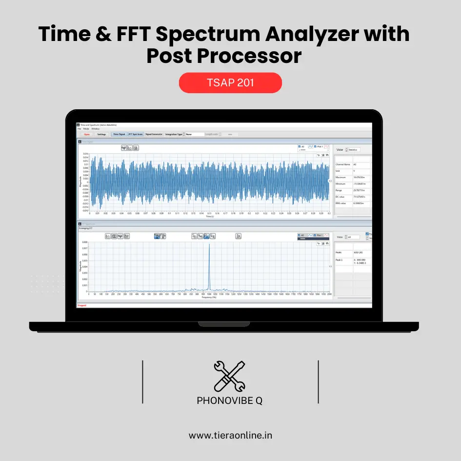 TSAP 201 -Time & FFT Spectrum Analyzer with Post Processor (Phonovibe Q)Use Cases Bump Test Product Development Off route Machine Vibration analysis. Drop Test Product Development & Research₹34,560View →
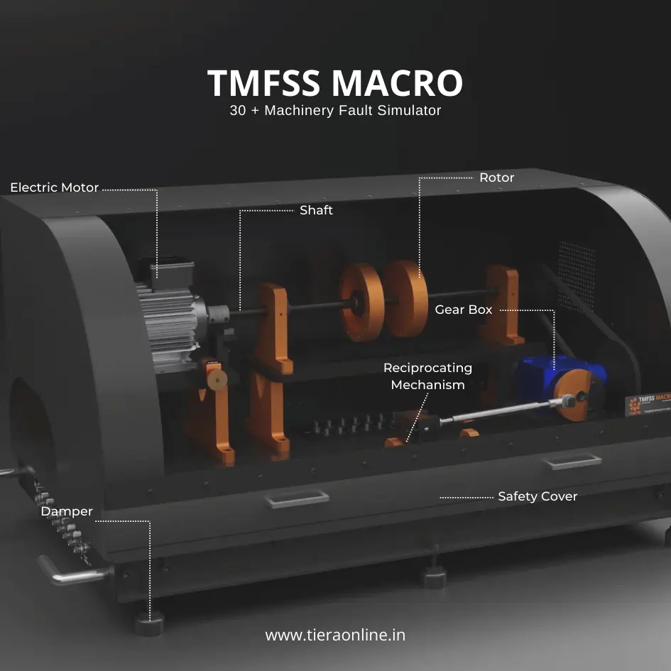 Machinery Fault Signature SimulatorTiera’s Machine Fault Simulator (TMFSS) is a valuable tool for industries and researchers, simulating over 30 real-world faults such as: Bearing faults: outer race defects, inner race defects, cage defects. Motor faults: stator faults, rotor faults, electrical unbalance. Gearbox faults: gear wear, misalignment, gear tooth damage. And more.₹13,53,600View →
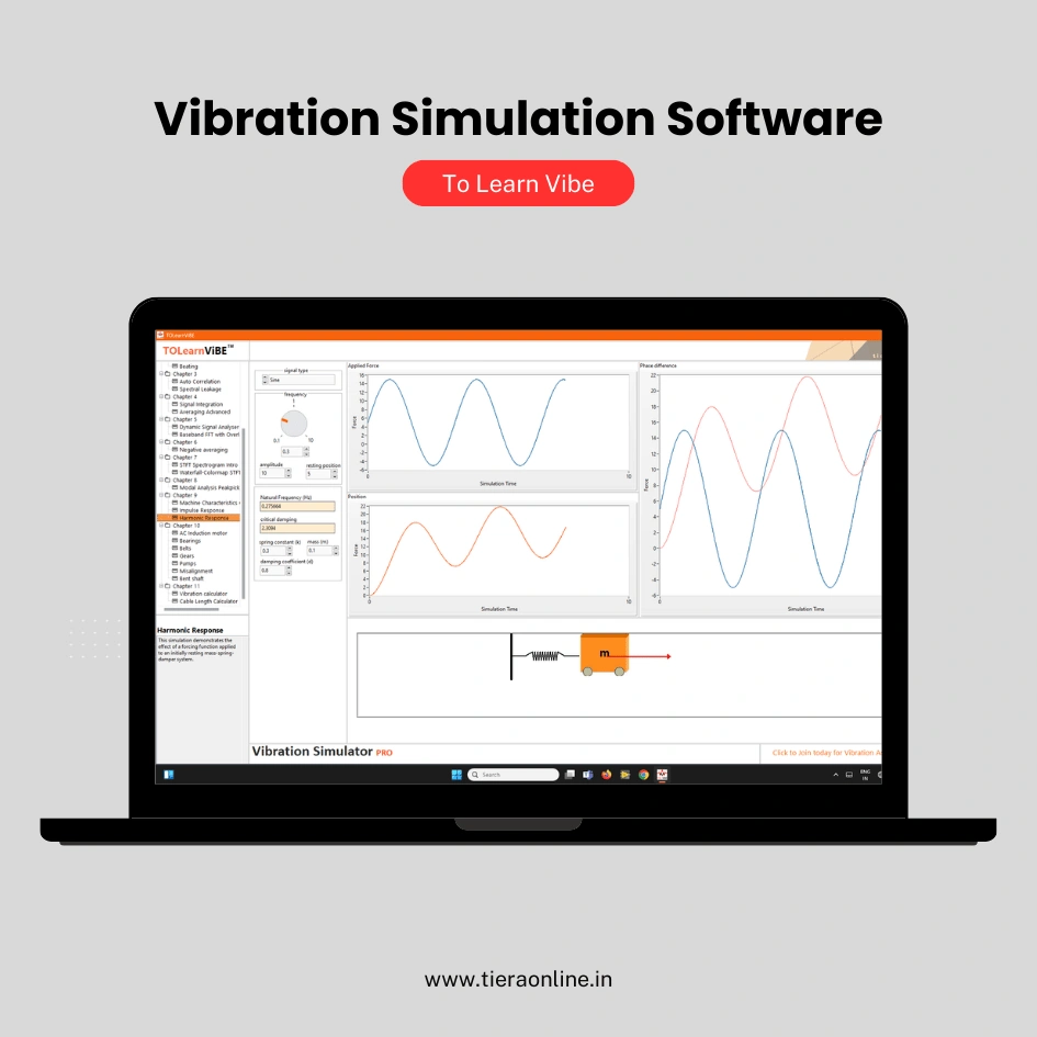 To Learn Vibe -Vibration Simulation Software Standard (Yearly Subscription)For comprehensive vibration analysis training, start with our To Learn Vibe software. Covering everything from basic to advanced vibration concepts, this software is designed to kickstart your career and enhance your expertise. Perfect for mastering fundamental and advanced vibration analysis, To Learn Vibe equips you with the knowledge and skills needed to excel in the field of vibration engineering.₹57,600View →
Use cases
Where this shows up in the field
When the sliders are not enough: make the fault real, capture it, analyse it
The simulator on this page teaches the shapes. TIERA builds the stack that teaches the substance. The TMFSS Machinery Fault Signature Simulator reproduces 30+ faults — unbalance, parallel and angular misalignment, foundation looseness, bearing defects, gearbox faults — physically, on a rigid benchtop rig with VFD speed control and a built-in tachometer, so every signature on this page can be created on demand and repeated tomorrow. Three sizes cover research labs (Macro) down to classrooms (Mini, Micro).
Capture and analysis complete the chain: a PhonoVibe 24-bit USB DAQ (2 to 16 channels, IEPE sensor power, simultaneous sampling) records the real waveform, and the bundled TVIB TSAP201 software computes the real spectrum — up to 102,400-line FFTs with the harmonic, band and sideband cursors this page's mini-DFT can only hint at. It is the same progression your analysts follow: recognise the shape here, then measure it for real.
- TMFSS Macro — 30+ repeatable fault conditions, add-on kits, technical note per fault
- PhonoVibe D/Q/O/HD — 24-bit USB DAQ, IEPE power, TEDS, TVIB TSAP201 bundled free
- TVIB — harmonic cursors, integration to velocity, order-based analysis of live signals
- TCAT-aligned training when the rig is part of a formal learning programme
Where this sits on the TIERA learning ladder.
The theory behind this article is covered free, in full, by the TIERA 101 primers: Vibration 101 (Foundations), Machinery Fault Diagnosis 101. They are self-paced, interactive, and end in an exam and a certificate.
The free 101 primers at 101.tieraonline.in cover the theory behind every slider on this page at no cost — they are learning material, not an accredited ISO certification. The formal TCAT programme (see /services) adds structured Cat-level coursework and proctored examinations at exams.tieraonline.in for teams that need assessed, certificated competence.
TIERA 101 is a free introductory primer, not an accredited ISO certification, and its hours do not count towards the formal training ISO 18436 requires.